Details
On 16 July 1945 the first detonation of a nuclear weapon occurred in the New Mexico desert at 5:29 AM. The code name for this test was Trinity and the device that was detonated was known as the gadget. This nuclear weapon was developed by the Manhattan project. The gadget was a plutonium implosion fission device. The name Trinity was chosen by Robert Oppenheimer, director of the Manhattan project. The concept for an implosion device is due to John von Neumann who was a major participant in the Manhattan Project. Although not directly employed by the Manhattan Project, the British scientist
Geoffrey Taylor performed important computations related to the mechanical energy released by a nuclear explosion. Taylor's computations ultimately made it possible to estimated the yield of the explosion using only a time-stamped sequence of photographs of the fireball and a self contained length scale.
An above ground nuclear explosion can be modeled as the sudden release of a finite amount of energy E from a point R=0. The location of the rapidly spreading, spherical shock wave at time t is functionally of the form R=R(t,E,ρ0,p0,e) where ρ0, p0 and e are respectively the density, pressure and energy per unit mass of the undisturbed atmosphere. Since this is a problem in mechanics, the fundamental dimensions are mass, length and time. These are independently spanned by the arrival time of the shock wave t, the energy released in the explosion E and undisturbed air density ρ0. Dimensional analysis implies that ρ0R5/(E t2)=f(p0R3/E,p0/(ρ0e)) for some function f. For a perfect gas p0/(ρ0e)=γ-1 where γ is the adiabatic gas constant. For a large explosion p0R3/E is small and its effect can be neglected. This leads to the relationship ρ0R5/(E t2)=g(γ) where g(γ) is a function that cannot be determined from dimensional analysis. An equivalent dimensional relationship is E = K(γ) ρ0R5t-2.
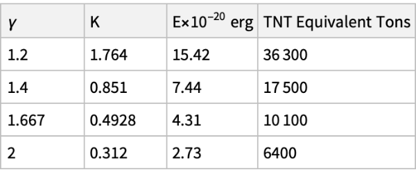
During the early stages of the second world ear (1940-1941) the sudden release of mechanical energy by a nuclear explosion was studied independently by the British scientist Geoffrey Taylor and the American scientist John von Neumann. They arrived at almost identical results and presented those results within days of one another in June 1941. In particular they both determined the form of the function K(γ) for a nuclear explosion modeled as a point release of intense energy. Their individual evaluations of K(γ) are presented here. Critical to both of their approaches was treating the explosion as a point rather than having some initial radius R0. In this respect a nuclear explosion was simpler to model than a large chemical explosion.
After the end of the second world war photographs of the Trinity test were declassified and made public. These photographs, which were made by J. Mack, were time stamped and contain a length scale. This made it possible for Geoffrey Taylor to determine the R-t blast wave relationship for the Trinity test. Specifically he found that the blast wave arrival time data almost exactly fell on the line defined by (5/2)log10R-log10t=11.915 where R is measured in cm and t is measured in sec. Taylor estimated the yield of the explosion to be 16,800 tons. John von Neumann's analysis combined with the arrival time data of the Trinity test leads to a similar result. The actual yield was about 20,000 tons. The Russian scientist L. I. Sedov performed similar computations although these did not become widely available till somewhat later.
A note about units is in order here. In the second world war scientists typically used to cgs system of units with centimeter for length, gram for mass and second for time. The unit of energy is the erg. One gram of TNT releases 1000 cal of energy which is equivalent to 4.186×10¹⁰ ergs. The British ton weighs 2240 pounds. One British ton of TNT releases 4.25×10¹⁶ ergs of energy. This value was used by Geoffrey Taylor in his conversion from ergs energy release to tons of energy release in a nuclear explosion.
In addition to the arrival time and distance of the blast wave the following photographs, historical computations and supporting measurements are available:
| "TrinityEarly" | blast photographs 0.24-1.93 msec |
| "Trinity016msec" | blast photograph at 16 msec |
| "Trinity025msec" | blast photograph at 25 msec |
| "Trinity053msec" | blast photograph at 53 msec |
| "Trinity062msec" | blast photograph at 62 msec |
| "Trinity090msec" | blast photograph at 90 msec |
| "KofGammaTaylor" | Taylor’s yield estimate |
| "KofGammaVonNeumann" | von Neumann’s yield estimate |
| "blastPressure" | recorded blast pressure |
![i1 = ResourceData[\!\(\*
TagBox["\"\<Trinity Nuclear Explosion Blast Wave\>\"",
#& ,
BoxID -> "ResourceTag-Trinity Nuclear Explosion Blast Wave-Input",
AutoDelete->True]\), "Trinity016msec"]; i2 = ResourceData[\!\(\*
TagBox["\"\<Trinity Nuclear Explosion Blast Wave\>\"",
#& ,
BoxID -> "ResourceTag-Trinity Nuclear Explosion Blast Wave-Input",
AutoDelete->True]\), "Trinity025msec"];
i3 = ResourceData[\!\(\*
TagBox["\"\<Trinity Nuclear Explosion Blast Wave\>\"",
#& ,
BoxID -> "ResourceTag-Trinity Nuclear Explosion Blast Wave-Input",
AutoDelete->True]\), "Trinity053msec"]; i4 = ResourceData[\!\(\*
TagBox["\"\<Trinity Nuclear Explosion Blast Wave\>\"",
#& ,
BoxID -> "ResourceTag-Trinity Nuclear Explosion Blast Wave-Input",
AutoDelete->True]\), "Trinity062msec"];
GraphicsGrid[{{i1, i2}, {i3, i4}}, ImageSize -> 600]](https://www.wolframcloud.com/obj/resourcesystem/images/25a/25a7f321-b803-4ebe-9a5b-d3828e133931/6892df310aa7f08f.png)
![pdata = ResourceData[\!\(\*
TagBox["\"\<Trinity Nuclear Explosion Blast Wave\>\"",
#& ,
BoxID -> "ResourceTag-Trinity Nuclear Explosion Blast Wave-Input",
AutoDelete->True]\), "blastPressure"];
data = Normal[Values[pdata]];
{t1, r1, p1} = Transpose[Select[data, First[#] == "Crusher Gauge" &]];
{t2, r2, p2} = Transpose[Select[data, First[#] == "Excess Velocity" &]];
{t3, r3, p3} = Transpose[Select[data, First[#] == "Foil Gauge" &]];
{t4, r4, p4} = Transpose[Select[data, First[#] == "Microbarograph" &]];
cg = Transpose[{r1, p1}]; ev = Transpose[{r2, p2}]; mb = Transpose[{r4, p4}];
pairs = Map[StringSplit[#, "-"] &, p3];
{p3min, p3max} = Transpose[Map[ToExpression, pairs]];
fgmin = Transpose[{r3, p3min}];
fgmax = Transpose[{r3, p3max}];
ListLogLogPlot[{cg, ev, fgmin, fgmax, mb}, Sequence[
PlotRange -> All, Axes -> False, Frame -> True, ImageSize -> 500, FrameLabel -> {"Range (yd)", "Pressure (psi)"}, AspectRatio -> 1, BaseStyle -> {FontSize -> 12}, PlotLegends -> {"Crusher Gauge", "Excess Velocity", "Foil Gauge min", "Foil Gauge max", "Microbarograph"}, PlotMarkers -> "OpenMarkers"]]](https://www.wolframcloud.com/obj/resourcesystem/images/25a/25a7f321-b803-4ebe-9a5b-d3828e133931/46e298d90db84c8b.png)
![taylorPressure = Table[{rangeyd, (1.45*10^-5) 9.3*10^22 (0.00125)/(0.9144*
rangeyd*100)^3}, {rangeyd, {50, 70, 200}}];
ListLogLogPlot[{cg, ev, taylorPressure}, Epilog -> {Line[Log[taylorPressure]]}, Sequence[
PlotRange -> All, Axes -> False, Frame -> True, ImageSize -> 500, FrameLabel -> {"Range (yd)", "Pressure (psi)"}, AspectRatio -> 1, BaseStyle -> {FontSize -> 12}, PlotLegends -> {"Crusher Gauge", "Excess Velocity", "Taylor Estimate"}, PlotMarkers -> "OpenMarkers"]]](https://www.wolframcloud.com/obj/resourcesystem/images/25a/25a7f321-b803-4ebe-9a5b-d3828e133931/7442336572af41ff.png)
![data = ResourceData[\!\(\*
TagBox["\"\<Trinity Nuclear Explosion Blast Wave\>\"",
#& ,
BoxID -> "ResourceTag-Trinity Nuclear Explosion Blast Wave-Input",
AutoDelete->True]\)];
tsec = 10^-3 Normal[data[All, 1]]; rcm = 10^2 Normal[data[All, 2]];
x = Log[10, tsec]; y = (5/2) Log[10, rcm];
theoreticalRt = Line[{{-4, -4 + 11.915}, {-1, -1 + 11.915}}];
ListPlot[Transpose[{x, y}], Sequence[
PlotRange -> All, AspectRatio -> 1, PlotRange -> All, Axes -> False, Frame -> True, FrameLabel -> {"\!\(\*SubscriptBox[\(log\), \(10\)]\)t (sec)", "(5/2)\!\(\*SubscriptBox[\(log\), \(10\)]\)R (cm)"}, Epilog -> theoreticalRt, ImageSize -> 400, BaseStyle -> {FontSize -> 12}]]](https://www.wolframcloud.com/obj/resourcesystem/images/25a/25a7f321-b803-4ebe-9a5b-d3828e133931/7d375be66799d14e.png)
![vonNeumannTable = ResourceData[\!\(\*
TagBox["\"\<Trinity Nuclear Explosion Blast Wave\>\"",
#& ,
BoxID -> "ResourceTag-Trinity Nuclear Explosion Blast Wave-Input",
AutoDelete->True]\), "KofGammaVonNeumann"]; Rasterize[vonNeumannTable,
ImageSize -> 300]](https://www.wolframcloud.com/obj/resourcesystem/images/25a/25a7f321-b803-4ebe-9a5b-d3828e133931/14ea7130dd484c5b.png)
![x1 = Normal@taylorTable[All, 1]; y1 = Normal@taylorTable[All, 4];
x2 = Normal@vonNeumannTable[All, 1]; y2 = Normal@vonNeumannTable[All, 4];
ListPlot[{Transpose[{x1, y1}], Transpose[{x2, y2}]}, Sequence[
PlotRange -> All, Axes -> False, Frame -> True, FrameLabel -> {"\[Gamma]: Adiabatic Constant", "Yield: TNT Equivalent Tons"}, ImageSize -> 400, AspectRatio -> 1,
PlotLegends -> {"Taylor", "von Neumann"}, BaseStyle -> {FontSize -> 12}]]](https://www.wolframcloud.com/obj/resourcesystem/images/25a/25a7f321-b803-4ebe-9a5b-d3828e133931/60e1f302a87b0f95.png)