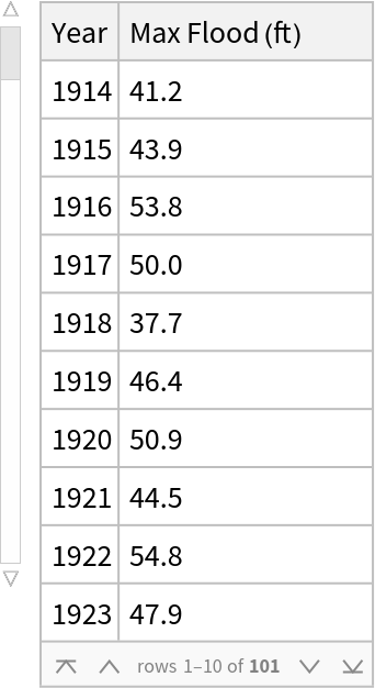
Maximum annual Mississippi River flood at Vicksburg, MS from 1922 to 2014
Examples
Visualizations (1)
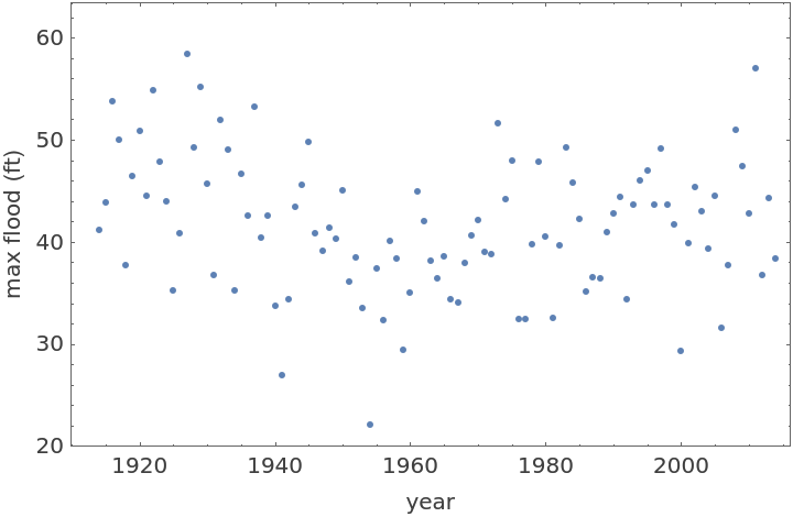
Plot the maximum river flood height by year:
Analysis (4)
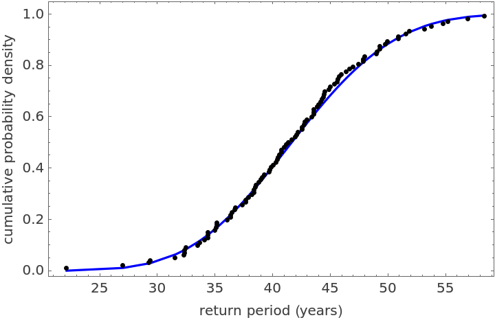
The river flood data are of the form annual block maxima and can be modeled by the MaxStableDistribution. Goodness of fit can be assessed by comparing the observed and theoretical cumulative distribution functions. By convention the observed cumulative probability density at year i is defined to be CDF(i)=(m+1)-1i where m=101 is the number of years that data were recorded. Plot the measured and theoretical values, respectively shown as points and a solid line:
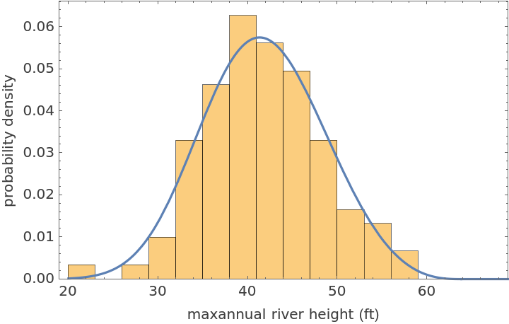
Create a Histogram of the observed maximum annual river heights compared to the theoretical probability density function for the MaxStableDistribution fit:
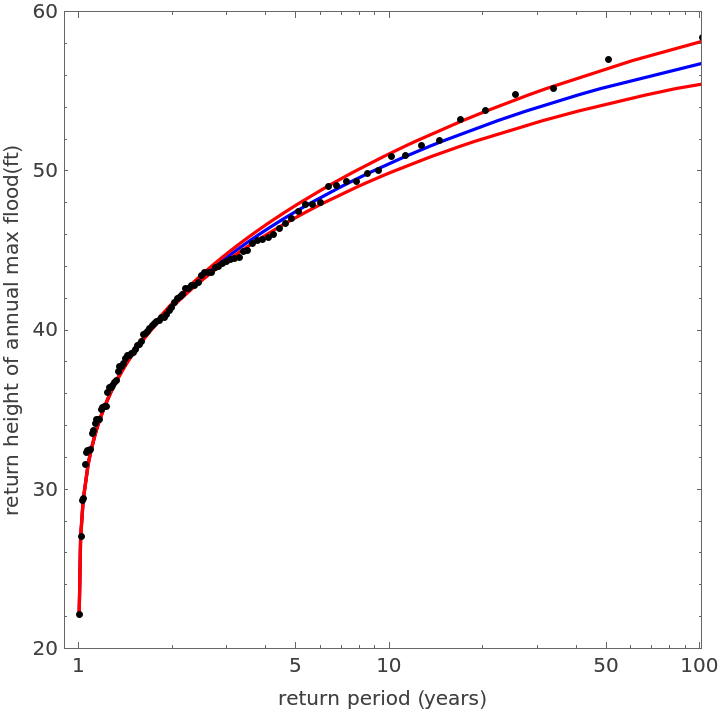
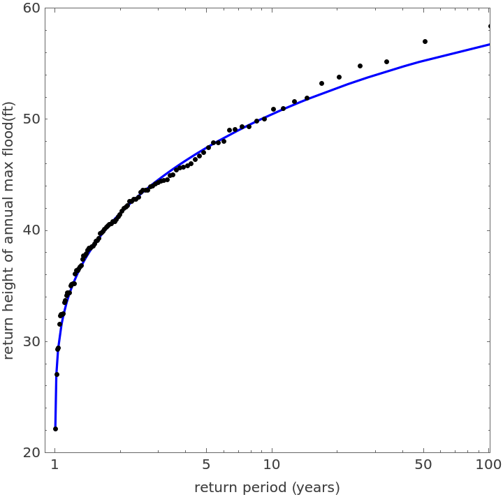
The return period (in years) to obtain a flood of height z is (1-CDF(z))-1. Compare the observed return periods to the theoretical return period values predicted by the MaxStableDistribution:
In order to further analyze the difference between observed and theoretical return periods, 95% error bars are placed on the theoretical curves. These error bars are computed using method of error calculation. In this technique the method of least squares refinement is used to place error bounds on the three fit parameters in the MaxStableDistribution. The upper and lower bounds on these three parameters are used in turn to compute an upper and lower range on the return period-return height curve. The resulting error bars are shown in red:
Bibliographic Citation
Marshall Bradley,
"Mississippi River Flood Heights"
from the Wolfram Data Repository
(2026)
Data Resource History
Publisher Information
![dataset = ResourceData[\!\(\*
TagBox["\"\<Mississippi River Flood Heights\>\"",
#& ,
BoxID -> "ResourceTag-Mississippi River Flood Heights-Input",
AutoDelete->True]\)];
ListPlot[dataset, Axes -> False, Frame -> True, PlotRange -> {20, 60},
FrameLabel -> {"year", "max flood (ft)"}]](https://www.wolframcloud.com/obj/resourcesystem/images/415/415a61be-3477-4a7e-bf1a-0566b73e7be9/153881c11ecec793.png)
![dataset = ResourceData[\!\(\*
TagBox["\"\<Mississippi River Flood Heights\>\"",
#& ,
BoxID -> "ResourceTag-Mississippi River Flood Heights-Input",
AutoDelete->True]\)];
year = Table[dataset[[i]][[1]], {i, 101}];
flood = Table[dataset[[i]][[2]], {i, 101}];
z = Sort[flood]; m = Length[flood];
edist1 = EstimatedDistribution[z, MaxStableDistribution[\[Mu], \[Sigma], k]];
{\[Mu]est, \[Sigma]est, kest} = {edist1[[1]], edist1[[2]], edist1[[3]]};
(*Ref: Coles(2004) chapter2, p. 36. *)
CDFMeasured = N[1/(m + 1) Table[i, {i, 1, m}]]; CDFModeled = Table[CDF[edist1, z[[i]]], {i, 1, m}];
ListPlot[{Transpose[{z, CDFMeasured}], Transpose[{z, CDFModeled}]}, Joined -> {False, True}, PlotStyle -> {{PointSize[0.01], Black}, Blue}, Axes -> False, Frame -> True, FrameLabel -> {"return period (years)", "cumulative probability density"}]](https://www.wolframcloud.com/obj/resourcesystem/images/415/415a61be-3477-4a7e-bf1a-0566b73e7be9/4fe73745d615560d.png)
![g1 = Histogram[z, {20, 70, 3}, "PDF", Axes -> False, Frame -> True, FrameLabel -> {"maxannual river height (ft)", "probability density"}];
g2 = Plot[PDF[edist1, h], {h, 20, 70}, Axes -> False, Frame -> True, FrameLabel -> {"max annual river height (ft)", "probability density"}];
Show[g1, g2]](https://www.wolframcloud.com/obj/resourcesystem/images/415/415a61be-3477-4a7e-bf1a-0566b73e7be9/0da1669da7a96d20.png)
![Tobs = 1/(1 - CDFMeasured); Tmod = 1/(1 - CDFModeled);
returnobs = Transpose[{Tobs, z}]; returnmod = Transpose[{Tmod, z}];
ListLogLinearPlot[{returnobs, returnmod}, PlotRange -> {{0.9, 101}, {20, 60}}, Joined -> {False, True}, PlotStyle -> {{PointSize[0.01], Black}, Blue}, AspectRatio -> 1, Axes -> False, Frame -> True, FrameLabel -> {"return period (years)", "return height of annual max flood(ft)"}]](https://www.wolframcloud.com/obj/resourcesystem/images/415/415a61be-3477-4a7e-bf1a-0566b73e7be9/3f3a74eda4baa93b.png)
![n\[Sigma] = 1.96;
del = CDFMeasured - CDFModeled; SSD = del . del; \[Sigma]calc = (SSD/(m - 3))^(1/2);
Clear[\[Mu], \[Sigma], k];
Arow = {D[E^-(1 + (k (x - \[Mu]))/\[Sigma])^(-1/k), \[Mu]], D[E^-(1 + (k (x - \[Mu]))/\[Sigma])^(-1/k), \[Sigma]], D[E^-(1 + (k (x - \[Mu]))/\[Sigma])^(-1/k), k]};
A = Table[
Arow /. {x -> z[[i]], \[Mu] -> edist1[[1]], \[Sigma] -> edist1[[2]],
k -> edist1[[3]]}, {i, 1, m}];
P = Inverse[
Transpose[A] . A]; COV = \[Sigma]calc^2 P; {\[Sigma]\[Mu], \[Sigma]\[Sigma], \[Sigma]k} = Sqrt@Diagonal[COV];
returnmin = {}; returnmax = {};
Do[cdfmin = CDF[MaxStableDistribution[\[Mu]est - n\[Sigma]*\[Sigma]\[Mu], \[Sigma]est - n\[Sigma]*\[Sigma]\[Sigma], kest - n\[Sigma]*\[Sigma]k], z[[j]]];
cdfmax = CDF[MaxStableDistribution[\[Mu]est + n\[Sigma]*\[Sigma]\[Mu], \[Sigma]est + n\[Sigma]*\[Sigma]\[Sigma], kest + n\[Sigma]*\[Sigma]k], z[[j]]];
If[cdfmin < 1, returnmin = Join[returnmin, {{1/(1 - cdfmin), z[[j]]}}]];
If[cdfmax < 1, returnmax = Join[returnmax, {{1/(1 - cdfmax), z[[j]]}}]];
, {j, 1, Length[z]}];
ListLogLinearPlot[{returnobs, returnmod, returnmin, returnmax}, PlotRange -> {{0.9, 101}, {20, 60}}, Joined -> {False, True, True, True}, PlotStyle -> {{PointSize[0.01], Black}, Blue, Red, Red}, AspectRatio -> 1, Axes -> False, Frame -> True, FrameLabel -> {"return period (years)", "return height of annual max flood(ft)"}]](https://www.wolframcloud.com/obj/resourcesystem/images/415/415a61be-3477-4a7e-bf1a-0566b73e7be9/6f6385dab5359ac2.png)