Wolfram Data Repository
Immediate Computable Access to Curated Contributed Data
Locations of amacrine cells (inhibitory interneurons in the retina) annotated with on/off marks
| In[1]:= |
| Out[1]= |  |
Summary of the spatial point data:
| In[2]:= |
| Out[2]= | 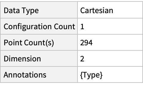 |
Plot the spatial point data:
| In[3]:= |
| Out[3]= | 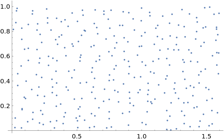 |
Plot annotated locations:
| In[4]:= |
| Out[4]= | 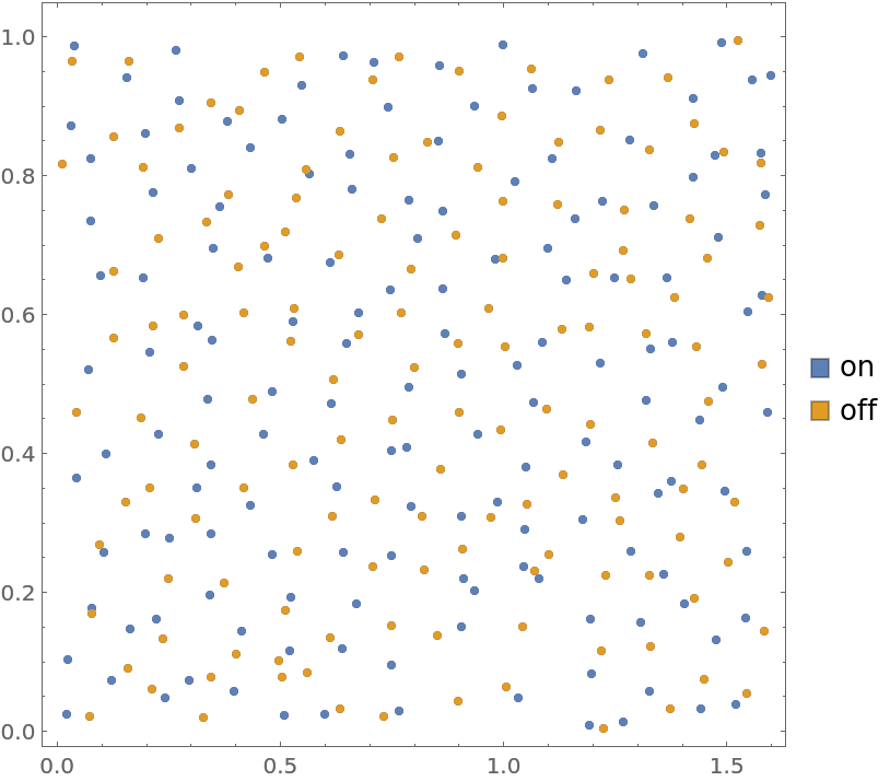 |
Compute probability of finding a point within given radius of an existing point - NearestNeighborG is the CDF of the nearest neighbor distribution:
| In[5]:= |
| Out[5]= |  |
| In[6]:= |
| Out[6]= |
| In[7]:= |
| Out[7]= | 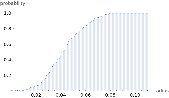 |
NearestNeighborG as the CDF of nearest neighbor distribution can be used to compute the mean distance between a typical point and its nearest neighbor - the mean of a positive support distribution can be approximated via a Riemann sum of 1- CDF. To use Riemann approximation create the partition of the support interval from 0 to maxR into 100 parts and compute the value of the NearestNeighborG at the middle of each subinterval:
| In[8]:= | ![step = maxR/100;
middles = Subdivide[step/2, maxR - step/2, 99];
values = nnG[middles];](https://www.wolframcloud.com/obj/resourcesystem/images/4ad/4ad6e4ec-7d2c-4dab-a7b0-f0afe268b48b/2536662d3a3fe7b0.png) |
Now compute the Riemann sum to find the mean distance between a typical point and its nearest neighbor:
| In[9]:= |
| Out[9]= |
Account for scale and units:
| In[10]:= |
| Out[10]= |
Test for complete spatial randomness:
| In[11]:= |
| Out[11]= |  |
Fit a Poisson point process to data:
| In[12]:= | ![Clear[\[Mu]];
EstimatedPointProcess[ResourceData[\!\(\*
TagBox["\"\<Sample Data: Amacrine Cells\>\"",
#& ,
BoxID -> "ResourceTag-Sample Data: Amacrine Cells-Input",
AutoDelete->True]\), "Data"], PoissonPointProcess[\[Mu], 2]]](https://www.wolframcloud.com/obj/resourcesystem/images/4ad/4ad6e4ec-7d2c-4dab-a7b0-f0afe268b48b/44c25448976ad5a0.png) |
| Out[13]= |
Gosia Konwerska, "Sample Data: Amacrine Cells" from the Wolfram Data Repository (2022)