Sample Data: Cancer Incidence

Source Notebook

Locations of cancer incidence annotated with larynx/lung marks

Details

Locations of cancer incidence in a polygonal observation region bounded by the region Rectangle[{343.45, 410.41}, {366.45, 431.79}] kilometers, annotated with larynx/lung marks.

Examples

Basic Examples (1) 

In[1]:=
ResourceData[\!\(\*
TagBox["\"\<Sample Data: Cancer Incidence\>\"",
#& ,
BoxID -> "ResourceTag-Sample Data: Cancer Incidence-Input",
AutoDelete->True]\), "Data"]
Out[1]=

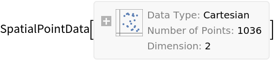
Summary of the spatial point data:

In[2]:=
ResourceData[\!\(\*
TagBox["\"\<Sample Data: Cancer Incidence\>\"",
#& ,
BoxID -> "ResourceTag-Sample Data: Cancer Incidence-Input",
AutoDelete->True]\), "Data"]["Summary"]
Out[2]=

Visualizations (3) 

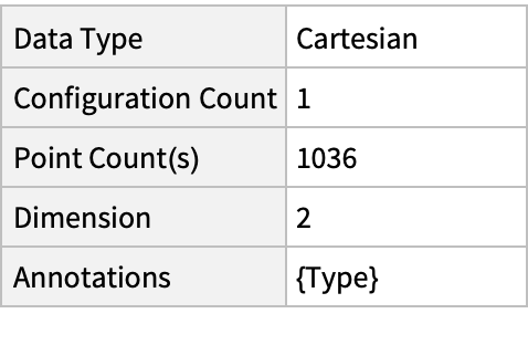
Plot the spatial point data:

In[3]:=
ListPlot[ResourceData[\!\(\*
TagBox["\"\<Sample Data: Cancer Incidence\>\"",
#& ,
BoxID -> "ResourceTag-Sample Data: Cancer Incidence-Input",
AutoDelete->True]\), "Data"]]
Out[3]=

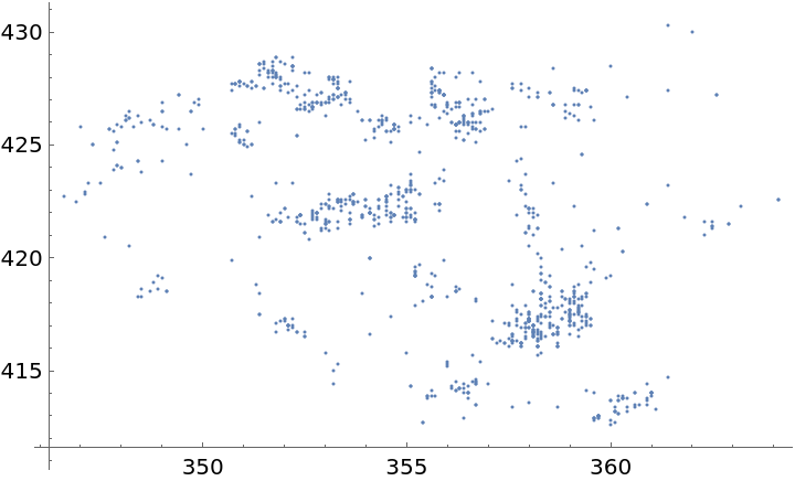
Visualize the data with the annotations:

In[4]:=
PointValuePlot[ResourceData[\!\(\*
TagBox["\"\<Sample Data: Cancer Incidence\>\"",
#& ,
BoxID -> "ResourceTag-Sample Data: Cancer Incidence-Input",
AutoDelete->True]\), "Data"], PlotLegends -> Automatic]
Out[4]=

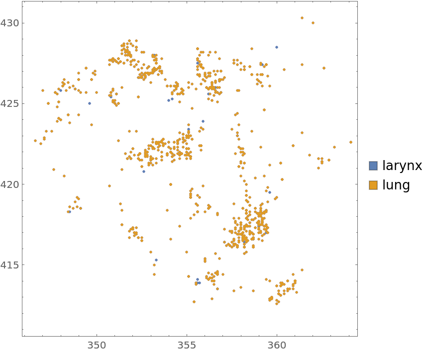
Visualize the smooth point density:

In[5]:=
density = SmoothPointDensity[ResourceData[\!\(\*
TagBox["\"\<Sample Data: Cancer Incidence\>\"",
#& ,
BoxID -> "ResourceTag-Sample Data: Cancer Incidence-Input",
AutoDelete->True]\), "Data"]]
Out[5]=
In[6]:=
Show[density["DensityVisualization"], ListPlot[ResourceData[\!\(\*
TagBox["\"\<Sample Data: Cancer Incidence\>\"",
#& ,
BoxID -> "ResourceTag-Sample Data: Cancer Incidence-Input",
AutoDelete->True]\), "Data"], PlotStyle -> Black]]
Out[6]=

Analysis (5) 

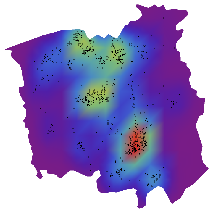
Compute probability of finding a point within given radius of an existing point - NearestNeighborG is the CDF of the nearest neighbor distribution:

In[7]:=
nnG = NearestNeighborG[ResourceData[\!\(\*
TagBox["\"\<Sample Data: Cancer Incidence\>\"",
#& ,
BoxID -> "ResourceTag-Sample Data: Cancer Incidence-Input",
AutoDelete->True]\), "Data"]]
Out[7]=
In[8]:=
maxR = nnG["MaxRadius"]
Out[8]=
In[9]:=
DiscretePlot[nnG[r], {r, 0, maxR, maxR/100}, PlotRange -> {0, 1}, AxesLabel -> {"radius", "probability"}]
Out[9]=

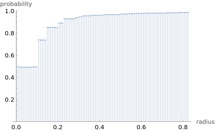
NearestNeighborG as the CDF of nearest neighbor distribution can be used to compute the mean distance between a typical point and its nearest neighbor - the mean of a positive support distribution can be approximated via a Riemann sum of 1-CDF. To use Riemann approximation create the partition of the support interval from 0 to maxR into 100 parts and compute the value of the NearestNeighborG at the middle of each subinterval:

In[10]:=
step = maxR/100;
middles = Subdivide[step/2, maxR - step/2, 100];
values = nnG[middles];

Now compute the Riemann sum to find the mean distance between a typical point and its nearest neighbor:

In[11]:=
Total[(1 - values)*step]
Out[11]=

Account for scale and units:

In[12]:=
 %*ResourceData[\!\(\*
TagBox["\"\<Sample Data: Cancer Incidence\>\"",
#& ,
BoxID -> "ResourceTag-Sample Data: Cancer Incidence-Input",
AutoDelete->True]\), "RegionScale"]
Out[12]=

Test for complete spatial randomness:

In[13]:=
SpatialRandomnessTest[ResourceData[\!\(\*
TagBox["\"\<Sample Data: Cancer Incidence\>\"",
#& ,
BoxID -> "ResourceTag-Sample Data: Cancer Incidence-Input",
AutoDelete->True]\), "Data"], {"PValue", "TestConclusion"}] // Column
Out[13]=

Gosia Konwerska, "Sample Data: Cancer Incidence" from the Wolfram Data Repository (2022)  

Data Resource History

Source Metadata

Publisher Information