Wolfram Data Repository
Immediate Computable Access to Curated Contributed Data
Datasets relating to Supreme Court cases from 1946 to present
Originator: Washington University in St. Louis School of Law
This is an adaptation of The Supreme Court Database maintained by Washington University in St. Louis ("WUSTL"). Two datasets are included: (1) a "case centered" dataset ("Case") that describes in each row of data a case decided by the court; and (2) a much larger "justice centered" dataset ("Justice") that describes in each row of data how a particular justice of that court voted on an issue within a case.
The WUSTL dataset provides extensive information on every decision of the United States Supreme Court since 1946 (excepting particularly insignificant determinations). The WUSTL website devoted to this data contains a lengthy explanation of the organization of the data and the meaning of each variable used therein. Thus, the column "issueArea" in the original WUSTL datasets has the same meaning and same encoding scheme as the column "issueArea" used in the two datasets presented here. Moreover, somewhat subjective determinations by WUSTL within the original datasets, such as whether a particular decision was "liberal" or "conservative," are not re-evaluated here; WUSTL's determinations are simply replicated. Research done using the original WUSTL datasets can thus be readily done using the representations of the data contained here.
This adaptation makes the WUSTL data more useful in several ways, however. First, the datasets here add columns with names ending in "S" and "F" that respectively provide a "short" and "full" explanation of the encoding system used by WUSTL for many of its columns. This permits users of the data to understand the meaning of (integer) values in those columns without extensive cross referencing with an online codebook provided by WUSTL that extends over dozens of web pages. Thus, in the original WUSTL dataset (and in the datasets here) the integer value 103 in the "petitioner" column would mean that the entity petitioning the Supreme Court for relief would be an "airplane manufacturer, or manufacturer of parts of airplanes." But one would not know this from the data value alone; one would have to consult a lengthy codebook. This dataset adds a column "petitionerS" that concisely identifies the petitioner as an "airplane manufacturer." It also adds a column "petitionerF" that more fully identifies the petitioner as an "airplane manufacturer, or manufacturer of parts of airplanes." The translation from WUSTL integer encodings to textual descriptions are taken from various spreadsheets not generally available but graciously provided by WUSTL to assist with this project. Thus, the textual descriptions of the data used here are fully consistent with the WUSTL understanding of the meaning of the integer codes.
Second, a few of the columns in the datasets refer to dates, persons and states for which there is more complete representation in the Wolfram Language through its framework for dealing with dates and its store of information on "Entities." Thus, dates of argument, reargument and decision are transformed here into DateObjects on which it is convenient to perform date arithmetic. And columns containing encodings of states and persons are augmented with columns with names ending in "E" that contain Entities. By way of example, the original data contains a column "respondentState" that contains an integer encoding of the state (or other geographic entity) in which the respondent resides (or is otherwise associated). For a particular case, it might thus contain a value 51. The datasets here add not only a column "respondentStateS" that contains "TX" (a postal abbreviation for Texas) and a column "respondentStateF" that contains "Texas" but also a column "respondentStateE" which contains Entity["AdministrativeDivision",{"Texas","UnitedStates"}] and whose properties can then be further queried using the Wolfram Language.
Users are cautioned that the justice centered dataset is over 1 gigabyte in size and it thus may take some time both to download and use the data on a local machine.
Retrieve the default content:
| In[1]:= |
| Out[1]= | 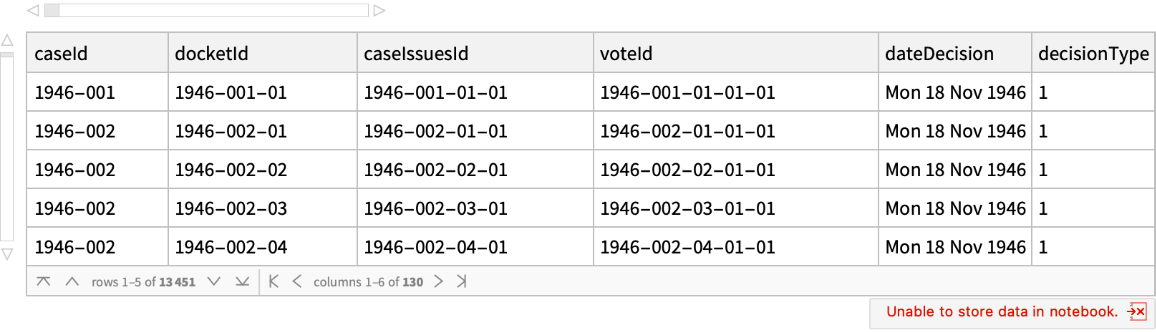 |
Retrieve the justice - centered dataset.
| In[2]:= |
| Out[2]= | 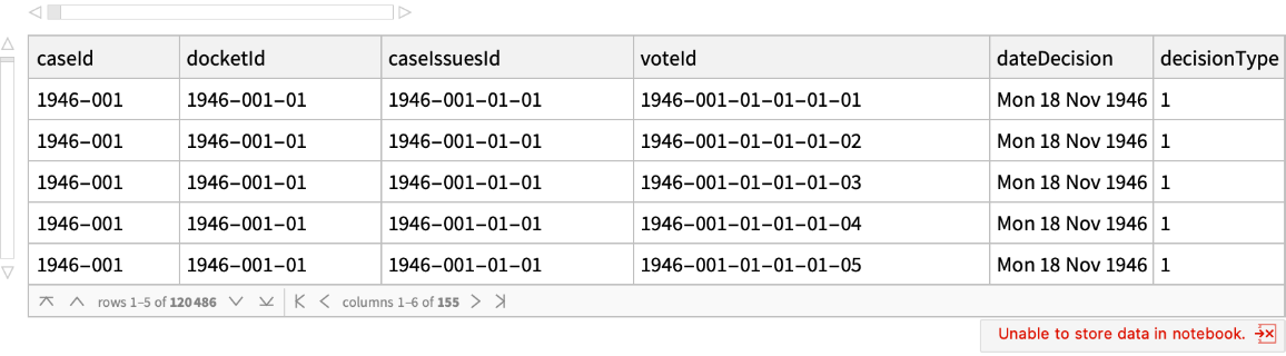 |
Create a table showing the columns of data available in each dataset.
| In[3]:= | ![caseKeys = Normal[Keys[
ResourceData[
"United States Supreme Court Decisions 1946-present"][1]]];
justiceKeys = Normal[Keys[$$Justice[1]]];
allKeys = Union[caseKeys, justiceKeys];](https://www.wolframcloud.com/obj/resourcesystem/images/813/81366ea3-ef31-4c06-813c-182874d9d2e0/2e68935cd33fec07.png) |
| In[4]:= | ![Row[Map[Grid[Join[{{"Column", "Case", "Justice"}}, #], Alignment -> Left, Dividers -> All, BaseStyle -> 10, Background -> {Lighter[Gray, 0.8], {Lighter[Blue, 0.8], {None}}}] &, Partition[
Table[{k, If[MemberQ[caseKeys, k], Style["\[Checkmark]", {Bold, Darker@Green}], Style["x", {Bold, Red}]], If[MemberQ[justiceKeys, k], Style["\[Checkmark]", {Bold, Darker@Green}], Style["x", {Bold, Red}]]}, {k, allKeys}], 39, 39, {1, 1}, {}]
], Spacer[6], Alignment -> {Left, Top}, BaselinePosition -> Top
]](https://www.wolframcloud.com/obj/resourcesystem/images/813/81366ea3-ef31-4c06-813c-182874d9d2e0/68f6b5ae00159d20.png) |
| Out[4]= | 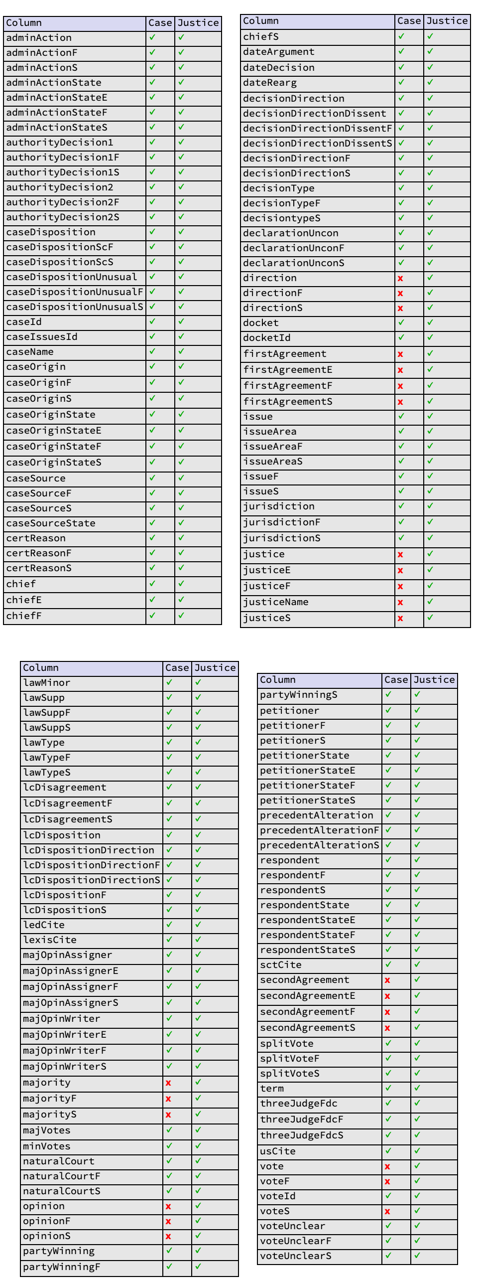 |
Find the first case in the dataset in which the petitioner was a manufacturer of airplanes and show information about the petitioner, the respondent and the issues
| In[5]:= | ![Query[SelectFirst[#petitioner == 103 &], {"petitioner", "petitionerS",
"petitionerF", "respondentF", "issueF"}][
ResourceData["United States Supreme Court Decisions 1946-present"]]](https://www.wolframcloud.com/obj/resourcesystem/images/813/81366ea3-ef31-4c06-813c-182874d9d2e0/0d8b36fa589f2a56.png) |
| Out[5]= | 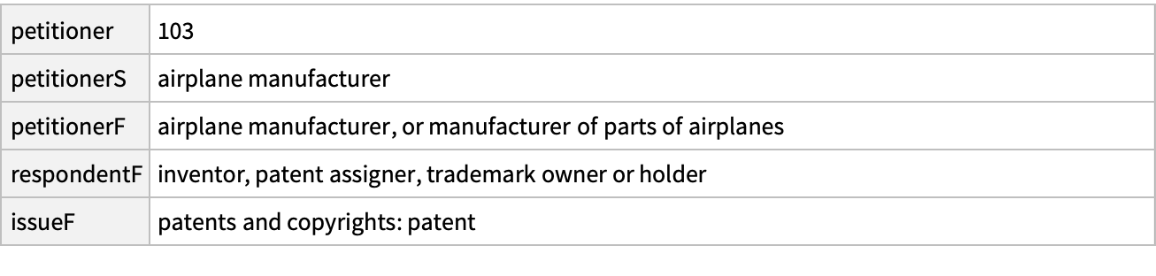 |
Compute the distribution of dispositions by the Supreme Court, sorted from most to least frequent:
| In[6]:= |
| Out[6]= | 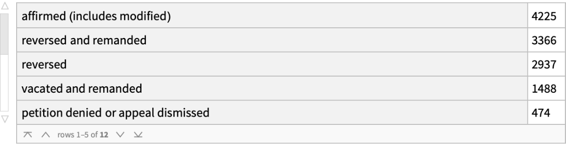 |
Compute a simplified version of dispositions by the Supreme Court, again sorted from most to least frequent.
| In[7]:= | ![simplifiedDisposition[disposition_] := Switch[disposition, "rev", "negative", "aff", "positive", "vac&rem", "negative", "aff&rev&rem", "mixed", "rev&rem", "negative", "vac", "negative", "petx/appx", "none", "aff&rev", "mixed", _, "none"]](https://www.wolframcloud.com/obj/resourcesystem/images/813/81366ea3-ef31-4c06-813c-182874d9d2e0/7ebe98a86ac5cabc.png) |
| In[8]:= |
| Out[8]= | 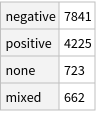 |
Although there are some cases decided by the Supreme Court that come within what is known as its "original jurisdiction" and are thus not decided beforehand by other courts, in most instances, cases come to the Supreme Court from what WUSTL reasonably terms a "source." We can use this information to determine the rate of positive, mixed, and negative Supreme Court dispositions based on the source court, restricting the search to courts that have had more than 250 cases reviewed. Assertions that the 9th Circuit is the most frequently reversed circuit appear to be true, although the Supreme Court treats decisions of state appellate courts even more negatively.
| In[9]:= | ![frequentCourts = Normal@Query[Counts/*Select[# > 100 &]/*Keys, #caseSourceF &][
ResourceData[
"United States Supreme Court Decisions 1946-present"]];
default = Normal@Query[
DeleteDuplicates/*(AssociationThread[#, 0] &), #caseDispositionScS &][
ResourceData[
"United States Supreme Court Decisions 1946-present"]];
simplifiedDefault = KeyMap[simplifiedDisposition, default];
Query[Query[SortBy[-#positive &]], Round[Normalize[#, Total], 0.001] &][
Query[Select[MemberQ[frequentCourts, #caseSourceF] &]/*
GroupBy[#caseSourceF &], GroupBy[simplifiedDisposition[#caseDispositionScS] &]/*(Merge[{#, simplifiedDefault}, First] &)/*
KeyTake[{"positive", "mixed", "negative", "none"}], Length][
ResourceData["United States Supreme Court Decisions 1946-present"]]]](https://www.wolframcloud.com/obj/resourcesystem/images/813/81366ea3-ef31-4c06-813c-182874d9d2e0/6763f1ad4d7d45b8.png) |
| Out[12]= | 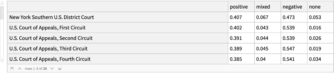 |
Which justice wrote the most majority opinions in each term? (A "term" is generally a year long period, starting in October, during which the Supreme Court decides cases, with a traditional break taken during the late summer of the following year).
| In[13]:= |
| Out[13]= | 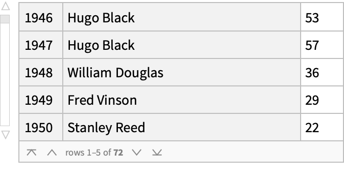 |
Can the vote of the justice vary within a case due to different issues being present? The answer is yes, but rarely.
| In[14]:= | ![simplifyVote[s_] := Switch[s, ("dissent" | "juisdictional dissent" | "dissent from denial of cert"), "dis", "voted w/ majority, plurality", "maj", ("special concurrence" | "regular concurrence"), "con", _, "other"];
defaultVote = AssociationThread[
Normal@Query[DeleteDuplicates, simplifyVote[#voteS] &][$$Justice], 0];
Query[Values/*Flatten/*Counts, Values][
Query[GroupBy[{#caseId &, #justice &}], All, SameQ @@ # &, #vote &][$$Justice]]](https://www.wolframcloud.com/obj/resourcesystem/images/813/81366ea3-ef31-4c06-813c-182874d9d2e0/4249b3ae8cbe6aa9.png) |
| Out[16]= | 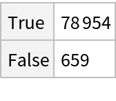 |
To what extent have different justices tended to go along with the majority view (maj), concurred (con), dissented (dis) or voted in other ways? The data here is sorted from highest fraction of majority view to lowest. The top three justices in this ranking were also Chief Justices. Justice William Douglas has the highest frequency of dissents (28.8%) with Justice Wiley Rutledge and John Harlan, II, having the highest rate of issuing concurring opinions.
| In[17]:= | ![rowNormalize[a_Association, f_ : (Round[#, 0.001] &)] := f@Normalize[a, Total]
rowNormalizeWithTotal[a_Association, f_ : (Round[#, 0.001] &)] := (Append[rowNormalize[a], "N" -> Total[a]])
Query[GroupBy[#justiceF &]/*Query[SortBy[-#maj &]], Counts/*(Merge[{#, defaultVote}, First] &)/*rowNormalizeWithTotal/*
KeyTake[{"maj", "con", "dis", "other", "N"}], simplifyVote[#voteS] &][$$Justice]](https://www.wolframcloud.com/obj/resourcesystem/images/813/81366ea3-ef31-4c06-813c-182874d9d2e0/05f5f9c868e214c7.png) |
| Out[19]= | 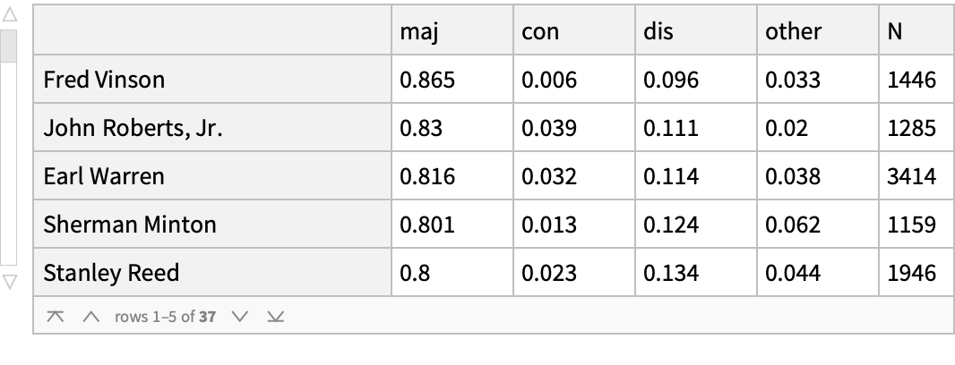 |
At what time of year does the Supreme Court issue decisions? One can see that opinions peak in June and that essentially no opinions are issued in August or September.
| In[20]:= |
| Out[20]= | 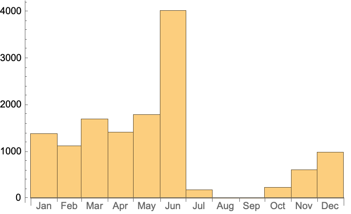 |
One can also study the pattern of agreement and disagreement among the justices. The Query below finds the rates of agreement (True) among the justices while William Rehnquist was Chief Justice. Legal scholars will not be surprised to find that the lowest rates of agreement were between Justices Antonin Scalia and Thurgood Marshall and the highest rates of agreement were between Thurgood Marshall and William Brennan.
| In[21]:= | ![With[{rehnquistCourtAgreement = Query[Select[#chiefF == "William Rehnquist" &]/*
GroupBy[#caseIssuesId &]/*Values/*Flatten/*Query[Merge[Counts]],
With[{a = Association[#]}, Association[(Sort[#] -> SameQ @@ Lookup[a, #]) & /@ Subsets[Keys[a], {2}]]] &, #justiceF -> simplifyVote[#voteS] &][$$Justice]}, SortBy[Last]@
KeyValueMap[#1 -> N[Round[#2[True]/Total[#2], 0.001]] &, Normal@rehnquistCourtAgreement]
]](https://www.wolframcloud.com/obj/resourcesystem/images/813/81366ea3-ef31-4c06-813c-182874d9d2e0/7f21ebfe12e2d6b4.png) |
| Out[21]= |  |
Consider the ideological proclivities of Justice Anthony Kennedy based on the issue area involved in the case. Conservative on criminal procedure and civil rights; liberal on taxes and the first amendment.
| In[22]:= | ![Query[Select[#justiceF == "Anthony Kennedy" && Not[MissingQ[#decisionDirectionF]] &]/*GroupBy[#issueAreaF &], Counts/*(Merge[{#, AssociationThread[{"liberal", "conservative", "unspecifiable"},
0]}, First] &)/*KeySort, #decisionDirectionF &][$$Justice]](https://www.wolframcloud.com/obj/resourcesystem/images/813/81366ea3-ef31-4c06-813c-182874d9d2e0/46bbfbb5c16cd303.png) |
| Out[22]= | 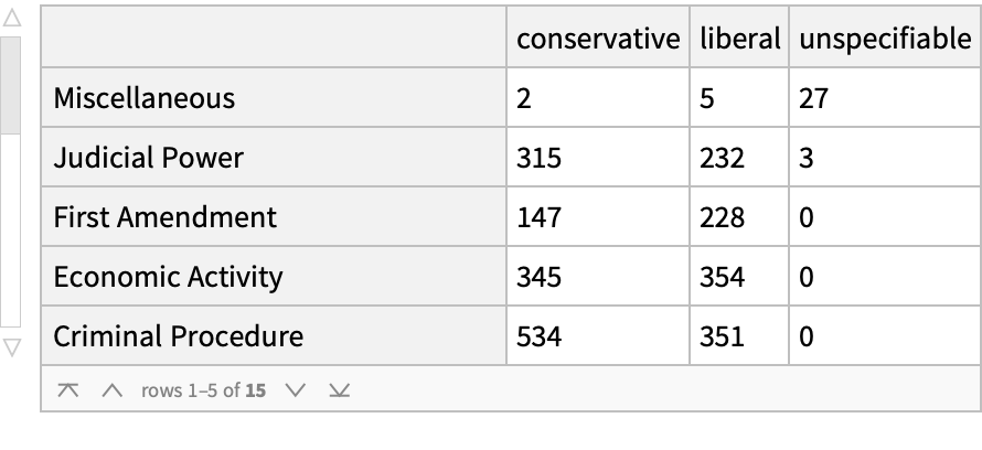 |
Here is a very simple effort to "machine learn" the voting patterns of the influential justice Anthony Kennedy based on 3985 issues that he decided. We first make sure we have data on the variable we want to classify and then we scramble the resulting dataset.
| In[23]:= | ![kennedyOnly = Query[Select[#justiceF == "Anthony Kennedy" && Not[MissingQ[#decisionDirectionF]] &]/*
RandomSample][$$Justice];](https://www.wolframcloud.com/obj/resourcesystem/images/813/81366ea3-ef31-4c06-813c-182874d9d2e0/7ed120bb2fa4a500.png) |
| In[24]:= |
| Out[24]= |
Separate the data into training and test data.
| In[25]:= |
Classify using just two columns : the type of law involved and the issue area involved.
| In[26]:= |
| Out[26]= |
See how we did on data the classifier did not use for training.
| In[27]:= |
| Out[27]= |
We gain some improvement over random guessing weighted by decision direction, but not a large amount. It's still hard to figure out the cases in which Justice Kennedy will lean liberal.
| In[28]:= |
| Out[28]= | 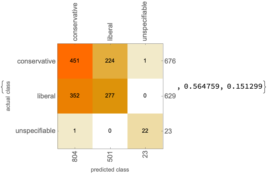 |
| In[29]:= |
Seth J. Chandler, "United States Supreme Court Decisions 1946-present" from the Wolfram Data Repository (2018)
https://creativecommons.org/licenses/by-nc/3.0/us/