Wolfram Data Repository
Immediate Computable Access to Curated Contributed Data
Locations of leukaemia in N.W. England from 1982 to 1998, annotated with age, gender, deprivation index, and subject type marks
| In[1]:= |
| Out[1]= | 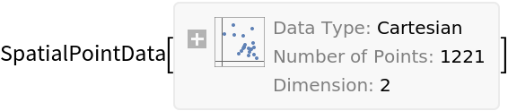 |
Summary of the spatial point data:
| In[2]:= |
| Out[2]= | 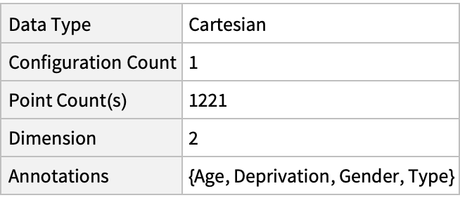 |
Plot the spatial point data:
| In[3]:= | ![Show[Graphics[{Opacity[.1], ResourceData[\!\(\*
TagBox["\"\<Sample Data: Leukaemia NW England\>\"",
#& ,
BoxID -> "ResourceTag-Sample Data: Leukaemia NW England-Input",
AutoDelete->True]\), "ObservationRegion"]}], ListPlot[ResourceData[\!\(\*
TagBox["\"\<Sample Data: Leukaemia NW England\>\"",
#& ,
BoxID -> "ResourceTag-Sample Data: Leukaemia NW England-Input",
AutoDelete->True]\), "Data"], AspectRatio -> Full], Axes -> True]](https://www.wolframcloud.com/obj/resourcesystem/images/817/8175c3ed-1685-4b48-ac02-0df03f408716/4e8dbcdbf8b55fc3.png) |
| Out[3]= | 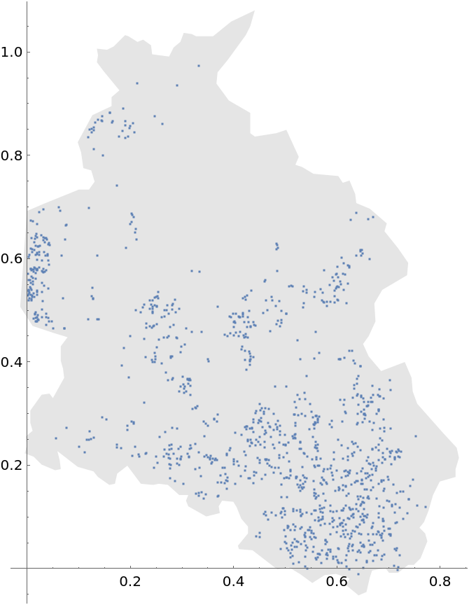 |
Plot the data annotated with gender (3rd annotation) marks:
| In[4]:= |
| Out[4]= | 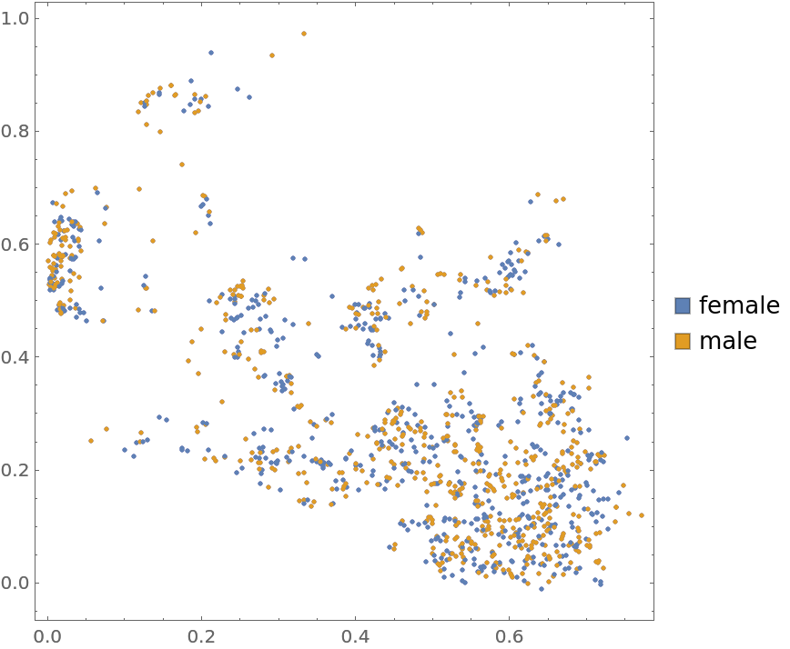 |
Plot the data annotated with type (4th annotation) marks:
| In[5]:= | ![PointValuePlot[ResourceData[\!\(\*
TagBox["\"\<Sample Data: Leukaemia NW England\>\"",
#& ,
BoxID -> "ResourceTag-Sample Data: Leukaemia NW England-Input",
AutoDelete->True]\), "Data"], {1 -> None, 2 -> None, 3 -> None, 4 -> Automatic}, PlotStyle -> {Magenta, Gray}, PlotLegends -> Automatic]](https://www.wolframcloud.com/obj/resourcesystem/images/817/8175c3ed-1685-4b48-ac02-0df03f408716/331e954aea2a1c87.png) |
| Out[5]= | 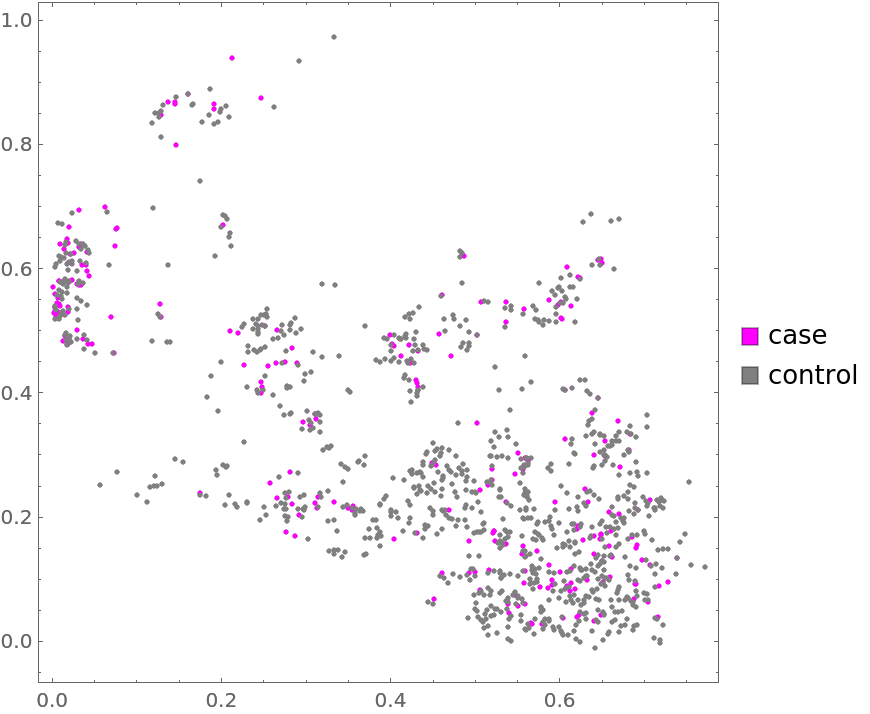 |
Compute probability of finding a point within given radius of an existing point - NearestNeighborG is the CDF of the nearest neighbor distribution:
| In[6]:= |
| Out[6]= |  |
| In[7]:= |
| Out[7]= |
| In[8]:= |
| Out[8]= | 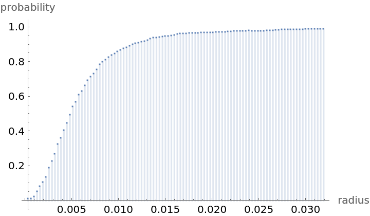 |
NearestNeighborG as the CDF of nearest neighbor distribution can be used to compute the mean distance between a typical point and its nearest neighbor - the mean of a positive support distribution can be approximated via a Riemann sum of 1- CDF. To use Riemann approximation create the partition of the support interval from 0 to maxR into 100 parts and compute the value of the NearestNeighborG at the middle of each subinterval:
| In[9]:= | ![step = maxR/100;
middles = Subdivide[step/2, maxR - step/2, 99];
values = nnG[middles];](https://www.wolframcloud.com/obj/resourcesystem/images/817/8175c3ed-1685-4b48-ac02-0df03f408716/7c0c416526087083.png) |
Now compute the Riemann sum to find the mean distance between a typical point and its nearest neighbor:
| In[10]:= |
| Out[10]= |
Test for complete spacial randomness:
| In[11]:= |
| Out[11]= |  |
Gosia Konwerska, "Sample Data: Leukaemia NW England" from the Wolfram Data Repository (2022)