Examples
Basic Examples (2)
Retrieve the model:
The icon:
Scope & Additional Elements (4)
Available content elements:
The available model types:
The operating point:
The parameters:
Visualizations (3)
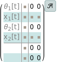
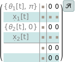
The numerical state space model:
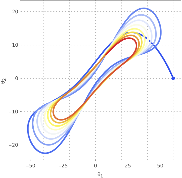
Simulate the pendulum's behaviour to some initial displacement angles:
Plot the trajectory in the configuration space:
Analysis (11)
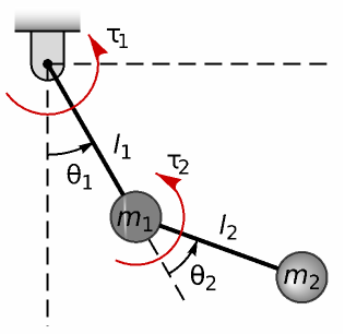
The model's equations and parameters:
An operating point about the inverted position:
Compute a numerical model for the new operating point:
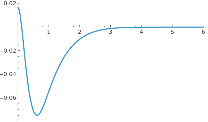
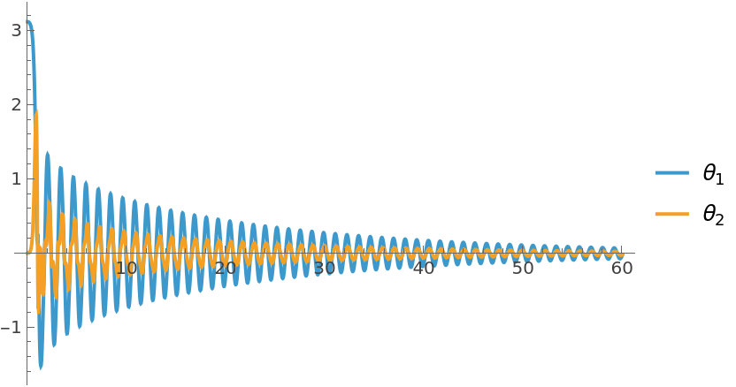
Its output response to a small deviation from the new equilibrium position:
The pendulum settles in its downward stable position:
The inverted double pendulum can be balanced using only τ1:
A specification for the controller design:
A state feedback controller:
Simulate the closed-loop system:
The pendulum is balanced in the upright position by the controller:
The control effort:
Bibliographic Citation
Suba Thomas,
"Double Pendulum Model"
from the Wolfram Data Repository
(2025)
Data Resource History
Publisher Information


![assm = ResourceData[\!\(\*
TagBox["\"\<Double Pendulum Model\>\"",
#& ,
BoxID -> "ResourceTag-Double Pendulum Model-Input",
AutoDelete->True]\)] /. ResourceData[\!\(\*
TagBox["\"\<Double Pendulum Model\>\"",
#& ,
BoxID -> "ResourceTag-Double Pendulum Model-Input",
AutoDelete->True]\), "Parameters"]](https://www.wolframcloud.com/obj/resourcesystem/images/84e/84e1ee8b-d2ac-43a1-bf62-83ab847be79d/31bdd1645a66226f.png)
![{eqns, pars} = assm = Table[ResourceData[\!\(\*
TagBox["\"\<Double Pendulum Model\>\"",
#& ,
BoxID -> "ResourceTag-Double Pendulum Model-Input",
AutoDelete->True]\), elems], {elems, {"Equations", "Parameters"}}]](https://www.wolframcloud.com/obj/resourcesystem/images/84e/84e1ee8b-d2ac-43a1-bf62-83ab847be79d/1e74fb6f8f0abbd2.png)

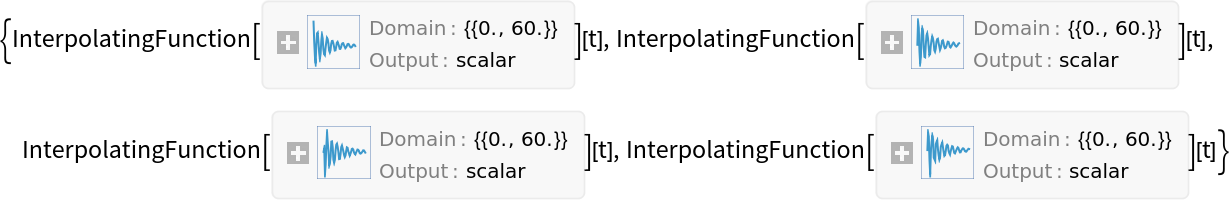
![ior = InputOutputResponse[{cd[{"ClosedLoopSystem", <|
"Merge" -> False|>}], {\[Pi] - 1 °}}, {0, 0}, {t, 0, 60}, "Data"]](https://www.wolframcloud.com/obj/resourcesystem/images/84e/84e1ee8b-d2ac-43a1-bf62-83ab847be79d/4a6dc38dfaa84a67.png)
![Grid[{Table[
Plot[r[[1]], {t, 0, 6}, PlotRange -> All, PlotLabel -> r[[2]]], {r, {ior["OutputResponse"]/Degree, {Subscript[\[Theta], 1], Subscript[\[Theta], 2]}}\[Transpose]}]}, Spacings -> {3, 0}]](https://www.wolframcloud.com/obj/resourcesystem/images/84e/84e1ee8b-d2ac-43a1-bf62-83ab847be79d/17b1c0f93adc8e7c.png)