Wolfram Data Repository
Immediate Computable Access to Curated Contributed Data
Locations of cattle herds in Cornwall (UK) that tested positive for bovine tuberculosis
| In[1]:= |
| Out[1]= |  |
Summary of the spatial point data:
| In[2]:= |
| Out[2]= | 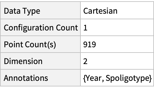 |
Plot the spatial point data:
| In[3]:= |
| Out[3]= | 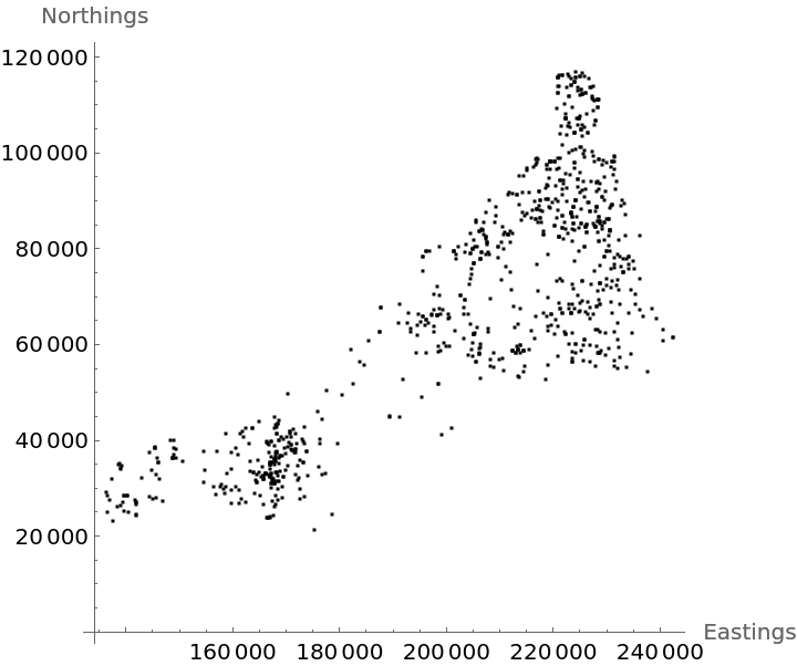 |
Visualize smooth point density:
| In[4]:= |
| Out[4]= |  |
| In[5]:= | ![Show[ContourPlot[density[{x, y}], {x, y} \[Element] ResourceData[\!\(\*
TagBox["\"\<Sample Data: Bovine Tuberculosis\>\"",
#& ,
BoxID -> "ResourceTag-Sample Data: Bovine Tuberculosis-Input",
AutoDelete->True]\), "ObservationRegion"], ColorFunction -> "Rainbow"], ListPlot[ResourceData[\!\(\*
TagBox["\"\<Sample Data: Bovine Tuberculosis\>\"",
#& ,
BoxID -> "ResourceTag-Sample Data: Bovine Tuberculosis-Input",
AutoDelete->True]\), "Data"], PlotStyle -> Black]]](https://www.wolframcloud.com/obj/resourcesystem/images/8c9/8c9cb285-6494-46ec-ae74-0e7285b67a25/140bca1e399a8590.png) |
| Out[5]= | 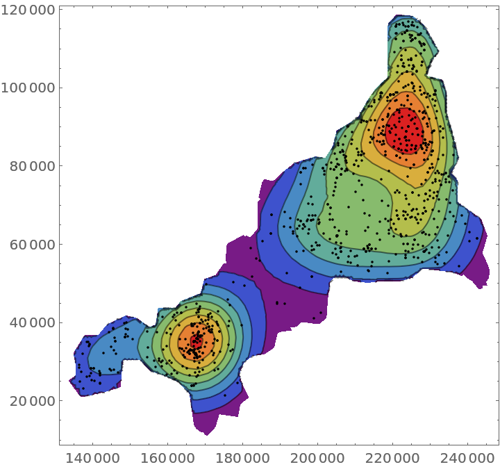 |
Compute probability of finding a point within given radius of an existing point - NearestNeighborG is the CDF of the nearest neighbor distribution:
| In[6]:= |
| Out[6]= | 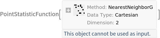 |
| In[7]:= |
| Out[7]= |
| In[8]:= |
| Out[8]= | 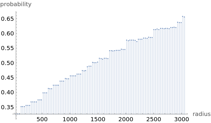 |
NearestNeighborG as the CDF of nearest neighbor distribution can be used to compute the mean distance between a typical point and its nearest neighbor - the mean of a positive support distribution can be approximated via a Riemann sum of 1- CDF. To use Riemann approximation create the partition of the support interval from 0 to maxR into 100 parts and compute the value of the NearestNeighborG at the middle of each subinterval:
| In[9]:= | ![step = maxR/100;
middles = Subdivide[step/2, maxR - step/2, 99];
values = nnG[middles];](https://www.wolframcloud.com/obj/resourcesystem/images/8c9/8c9cb285-6494-46ec-ae74-0e7285b67a25/074bb6760e1845de.png) |
Now compute the Riemann sum to find the mean distance between a typical point and its nearest neighbor:
| In[10]:= |
| Out[10]= |
Test for complete spatial randomness:
| In[11]:= |
| Out[11]= |  |
Gosia Konwerska, "Sample Data: Bovine Tuberculosis" from the Wolfram Data Repository (2022)