A Catalog of Jeffreys Priors

A catalog of Jeffreys prior probability distributions for use in a Bayesian statistical analysis

Details

A primary aim of a Bayesian analysis of a measurement is to make inference about the unkown parameters in model that properly reflect uncertainty in the measurement process. Bayes theorem is the proper calculus for doing this. A Bayesian analysis involves four interelated quantities. They are the prior probability distribution of the unknown parameters, the likelihood of the data given a knowledge of the parameters, the eveidence of the data and the posterior. distribution of the unknown parameters. Bayes theorem provides the relationship between these four quantities. If θ denotes an unknown parameter or vector of parameters and D denotes data then Bayes theorem requires that the posterior probability distribution P(θ|D)=E^-1f(θ)L(D|θ) where L(D|θ) is the likelhood of the data for given θ, f(θ) is the prior on θ and E is the evidence. The eveidence is just the normalization factor

where the range of integration is across all possible values of the parameterθ.

The investigator must supply the likelihood and prior. Bayes theorm does not tell us what they are. The likelihood function function L(D|θ) is ideally determined by the nature of the measurement, measurement instrument and the types of errors incurred. The prior encaulates what is known about the parameter vector θ before logically acquiring the data. The Jeffreys prior was proposed by Sir Harold Jeffreys as procedure for determining a prior probability distribution f(θ) that is invariant under a reparmeterization of the problem. For example,the normal probability distribution is usually described in terms of the standard deviation σ. But htere is no reason why the distribution could not be described in terms of the precision h=σ^-1. If one chooses a uniform prior for σ then reparametrization in terms of h causes dificulties. This problem can be overcome by choosing a Jeffreys prior for σ instead of a uniform prior.

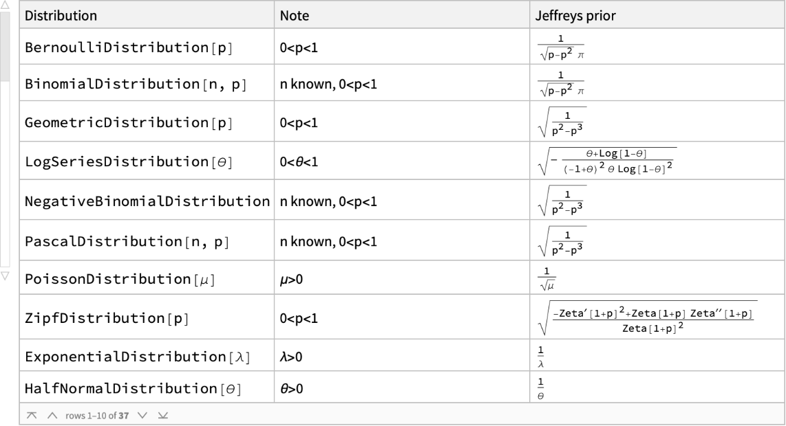
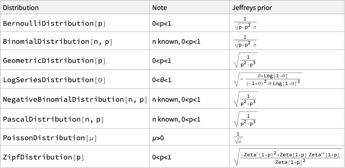
The Jeffreys prior f(θ) is defined as being proportional to the square root of the absoulte value of determinant of the Fisher information matrix ℐ(θ). In one dimension ℐ(θ)=-E[∂²log L(x|θ)/∂θ²] where x is data and the expecation is taken across the data x. For example consider the case of a single data sample from an an exponential distribution with unkown scale θ. Then the likelihood of the data sample is L(x|θ)=θ^-1exp(-x/θ). The Jeffreys prior in this case is f(θ)=θ^-1, 0<θ<θ. This is not proper probability density function and is in fact referred to as an improper prior. In a practical application one defines a finite range for θ and normalizes f(θ) to achieve f(θ)=(log(θ_max/θ_min))¹θ^-1 where θ_min<θ<θ_max.

For multidimensional problems with J parameters, the Fisher information matrix is the J×J matrix with elements

where the expectation is taken with respect to the data. An interpretation of the Fisher information is as follows. Second derivatives are measures of the curvature of a function. Thus if the second derivative of a function is large and negative corresponding to a maximum then the corresponding information will be large and positive. A Jeffreys prior tends to give more weight to parameter values corresponding to data with high information. This tends to cause the influence of the prior and data to coincide.

Harold Jeffreys in his writing motivated what we now call the Jeffreys prior in the following way. The likelihood of a data value x drawn from a normal distribution with mean μ and standard deviation σ is L(x|μ,σ)=(2π σ²)^-1/2exp(-(x-μ)²/2σ²). However it is just as correct to work in terms of the precision h=σ^-1. In this case the likelihood is L(x|μ,h)=(h²/2π)^1/2exp(-(x-μ)²h²/2)). Changing varaibles from σ to h should not change the results of a Bayesian inference. This suggests that there is a probability density function f(h) such that P(h₁<h<h₁+δ h)=f(h)δ h=P(σ₁>σ>σ₁-δ σ)∝f(σ) δ σ. The only function which satisifies f(h)δ h∝f(σ)δ σ is the function f(h)∝1/h and f(σ)∝1/σ. The requirement that our statistical inference remains invariant under the change of variable h=σ^-1 for the normal proability density law leads to the prior f(σ)=σ^-1.

The probability density function for several important probability distributions such as the normal, Cauchy and Student T can be written in terms of a location paramter μ and a scale parameter σ. The probability density for one of these distributions is g(x|μ,σ)=σ^-1ϕ((x-μ)/σ) where ϕ(ξ) is a dimensionless function. For the normal and Cauchy distributions respectively ϕ(ξ)=(2π)^-1/2exp(-ξ²/2) and ϕ(ξ)=π^-1(1+ξ²)^-1. These types of probability distributions have the same Jeffreys priors. If the location parameter μ is held constant then the Jeffreyrs prior is f(σ)=σ^-1. If the scale parameter σ is held constant then the Jeffreys prior is f(μ)=1. The joint Jeffreys prior is f(μ,σ)=σ^-2. In making these computations it has been assumed that the parameters of interest are μ and σ. Some authors assume that μ and σ² are the parameters of interest. This leads to different results.

Many problems in statistical inference involve a data sample D=x₁,x₂…x_n in which the data samples are independently drawn from a distribution with probability density g(x|θ). the joint likelihood of the data sample is L(D|θ)=∏i=1ng(x_i|θ). In this case the Jeffreys prior for the joint likelihood is the same as the Jeffreys prior for the individual data samples. This follows from the fact that log L(D|θ)=∑i=1nlog g(x_i|θ).

The Jeffreys prior f(σ)=σ^-1 for a scale parameter σ is equivalent to assuming that the prior on the scale scale parameter is uniformly distributed on a logarithmic scale. Consider the problem of estimating the mass of a star. On prior knowledge it is known that the mass M is greater than 1/1000 the mass of the sun but less than 1000 times the mass of the sun. The range of possible values for M is 10^-3M_sun<M<10³M_sun. Assuming that on prior knowledge that M is uniforly distrubted on (10^-3M_sun,10³M_sun) puts too much emphasis on larger values. Using the Jeffreys prior f(M)∝M^-1 overcomes this difficulty.

(3 columns, 37 rows)

Examples

Basic Examples (2)

In[1]:=

$ResourceData[\!$\* TagBox["\"\<A Catalog of Jeffreys Priors\>\"", #& , BoxID -> "ResourceTag-A Catalog of Jeffreys Priors-Input", AutoDelete->True]$]$

Out[1]=

Display the Jeffreys priors for the discrete probability density functions:

In[2]:=

$ResourceData[\!$\* TagBox["\"\<A Catalog of Jeffreys Priors\>\"", #& , BoxID -> "ResourceTag-A Catalog of Jeffreys Priors-Input", AutoDelete->True]$][1 ;; 8]$

Out[2]=

Scope & Additional Elements (1)

Retrieve the data and display the Jeffreys priors for the single parameter exponential family probability density functions:

In[3]:=

$rdata = ResourceData[\!$\* TagBox["\"\<A Catalog of Jeffreys Priors\>\"", #& , BoxID -> "ResourceTag-A Catalog of Jeffreys Priors-Input", AutoDelete->True]$][9 ;; 12]$

Out[3]=

Visualizations (1)

Plot the Jeffreys priors for the binomial and geometric probability density functions:

In[4]:=

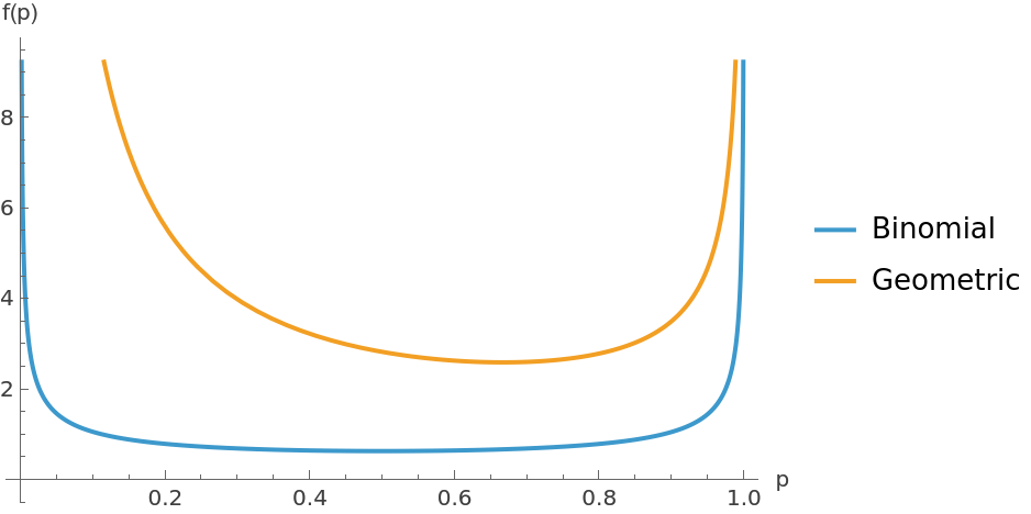
$rdata = ResourceData[\!$\* TagBox["\"\<A Catalog of Jeffreys Priors\>\"", #& , BoxID -> "ResourceTag-A Catalog of Jeffreys Priors-Input", AutoDelete->True]$]; fBinomial[p_] := Normal@rdata[All, 3][[2]]; fGeoemtic[p_] := Normal@rdata[All, 3][[3]]; Plot[{fBinomial[p], fGeoemtic[p]}, {p, 0.001, 0.999}, AxesLabel -> {"p", "f(p)"}, PlotLegends -> {"Binomial", "Geometric"}]$

Out[5]=

Analysis (2)

Obtain the Jeffreys prior for the exponential distribution in terms of the timescale parameter τ:

In[6]:=

$case = 9; rdata = ResourceData[\!$\* TagBox["\"\<A Catalog of Jeffreys Priors\>\"", #& , BoxID -> "ResourceTag-A Catalog of Jeffreys Priors-Input", AutoDelete->True]$]; rdata[All, 3][[case]] /. {\[Lambda] -> \[Tau]}$

Out[7]=

For a scale parameter of a sampling distribution the Jeffreys prior is often an improper probability distribution. If a single observation of the data is available then this observation and the Jeffreys prior can often be combined to produce a normalized prior distribution which can be used as the beginning point for a Bayesian analysis. As an example, the model of radioactive decay is the exponential distribution p(t|τ)=τ^-1exp(-t/τ) where t is an observed decay time with 0<t<∞. The parameter τ is the mean lifetime. The Jeffreys prior for τ is μ(τ)∝τ^-1 and is improper. The evidence of a data sample t in light of the prior is . 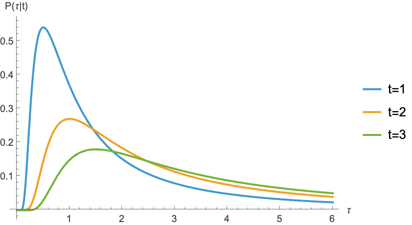The posterior distribution for τ follows from Bayes' theorem and is P(τ|t)=𝒩^-1τ^-2exp(-t/τ)=t τ^-2exp(-t/τ). For any observation t>0, P(τ|t) as defined here is a normalized probability density function.

In the following example the posterior distribution P(τ|t) is computed for observed decay times of 1, 2 and 3 sec:

In[8]:=

$t1 = 1.0; t2 = 2.0; t3 = 3; post[\[Tau]_, t_] := t*\[Tau]^-2*Exp[-t/\[Tau]] Plot[{post[\[Tau], t1], post[\[Tau], t2], post[\[Tau], t3]}, {\[Tau], 0.01, 6}, PlotRange -> All, AxesLabel -> {"\[Tau]", "P(\[Tau]|t)"}, PlotLegends -> {"t=1", "t=2", "t=3"}]$

Out[10]=

Bibliographic Citation

Marshall Bradley, "A Catalog of Jeffreys Priors" from the Wolfram Data Repository (2026)

Data Resource History

Date Created: 23 April 2026

Source Metadata

Citation: Source, reference or citation information

Publisher Information

Prepared for the Wolfram Data Repository By: Marshall Bradley
Publisher of Record: Marshall Bradley