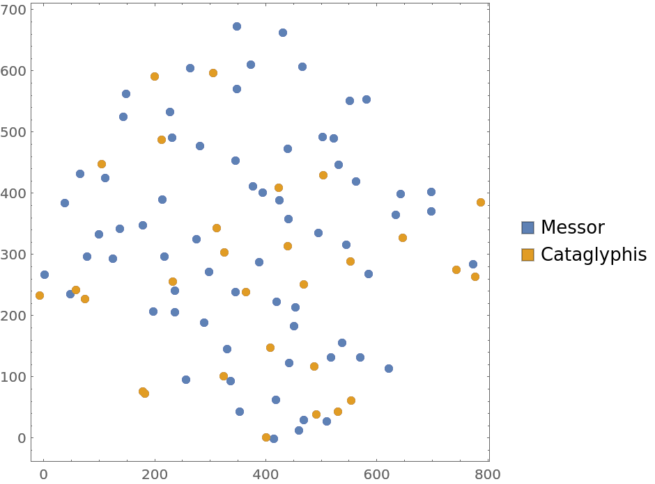
Locations of ant nests with marks denoting two types of species

Details

Locations of ant nests in the observation region Rectangle[{-7, -1}, {787, 673}] in feet, annotated with species Cataglyphis/Messor.

Examples

Basic Examples (3) 

Retrieve the data:

In[1]:=
ResourceData[\!\(\*
TagBox["\"\<Ant Nests\>\"",
#& ,
BoxID -> "ResourceTag-Ant Nests-Input",
AutoDelete->True]\)]
Out[1]=

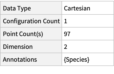
Summary of the spatial point data:
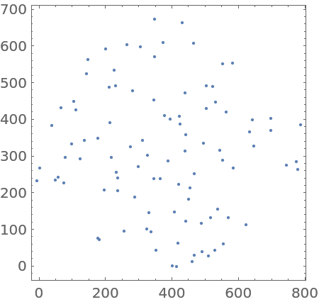
In[2]:=
ResourceData[\!\(\*
TagBox["\"\<Ant Nests\>\"",
#& ,
BoxID -> "ResourceTag-Ant Nests-Input",
AutoDelete->True]\), "Data"]["Summary"]
Out[2]=

Plot the points:

In[3]:=
ListPlot[ResourceData[\!\(\*
TagBox["\"\<Ant Nests\>\"",
#& ,
BoxID -> "ResourceTag-Ant Nests-Input",
AutoDelete->True]\), "Data"], Frame -> True, AspectRatio -> 1]
Out[3]=

Scope & Additional Elements (1) 

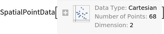
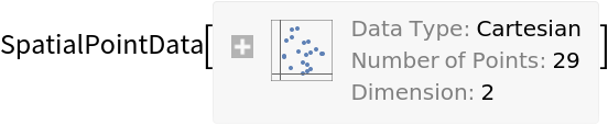
Select subsets based on the species type:

In[4]:=
messor = SpatialPointSelect[ResourceData[\!\(\*
TagBox["\"\<Ant Nests\>\"",
#& ,
BoxID -> "ResourceTag-Ant Nests-Input",
AutoDelete->True]\), "Data"], #Species == "Messor" &]
Out[4]=
In[5]:=
cataglyphis = SpatialPointSelect[ResourceData[\!\(\*
TagBox["\"\<Ant Nests\>\"",
#& ,
BoxID -> "ResourceTag-Ant Nests-Input",
AutoDelete->True]\), "Data"], #Species == "Cataglyphis" &]
Out[5]=

Visualizations (1) 

Plot locations with information about species:

In[6]:=
PointValuePlot[ResourceData[\!\(\*
TagBox["\"\<Ant Nests\>\"",
#& ,
BoxID -> "ResourceTag-Ant Nests-Input",
AutoDelete->True]\), "Data"], PlotLegends -> Automatic]
Out[6]=

Analysis (4) 

Test for complete spacial randomness:

In[7]:=
SpatialRandomnessTest[ResourceData[\!\(\*
TagBox["\"\<Ant Nests\>\"",
#& ,
BoxID -> "ResourceTag-Ant Nests-Input",
AutoDelete->True]\), "Data"], {"PValue", "TestConclusion"}]
Out[7]=

Fit a hard core point process to data:

In[8]:=
EstimatedPointProcess[ResourceData[\!\(\*
TagBox["\"\<Ant Nests\>\"",
#& ,
BoxID -> "ResourceTag-Ant Nests-Input",
AutoDelete->True]\), "Data"], HardcorePointProcess[\[Mu], r, 2]]
Out[8]=

Compute probability of finding a point within given radius of an existing point - NearestNeighborG is the CDF of the nearest neighbor distribution:

In[9]:=
nnG = NearestNeighborG[ResourceData[\!\(\*
TagBox["\"\<Ant Nests\>\"",
#& ,
BoxID -> "ResourceTag-Ant Nests-Input",
AutoDelete->True]\), "Data"]]
Out[9]=
In[10]:=
DiscretePlot[nnG[r], {r, 0.01, nnG["MaxRadius"], 1}, AxesLabel -> {"radius", "probability"}]
Out[10]=

Mean distance between a typical point and its nearest neighbor (for positive support distribution can be approximated via a Riemann sum of 1-CDF):

In[11]:=
step = nnG["MaxRadius"]/100.;
partition = Table[{k, k + step}, {k, 0, nnG["MaxRadius"], step}];
values = nnG[Mean /@ partition];
In[12]:=
Total[(1 - values)*step]*ResourceData[\!\(\*
TagBox["\"\<Ant Nests\>\"",
#& ,
BoxID -> "ResourceTag-Ant Nests-Input",
AutoDelete->True]\), "RegionUnit"]
Out[12]=

Gosia Konwerska, "Ant Nests" from the Wolfram Data Repository (2021)  

Data Resource History

Source Metadata

Publisher Information
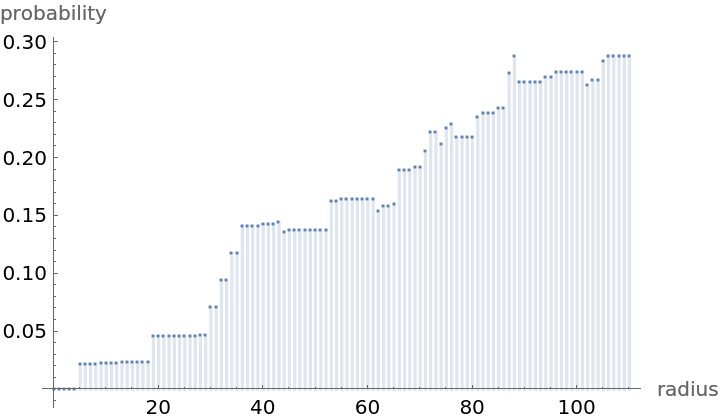