Wolfram Data Repository
Immediate Computable Access to Curated Contributed Data
Fire insurance claims in Denmark from Thursday 3rd January 1980 until Monday 31st December 1990
| In[1]:= |
| Out[1]= |
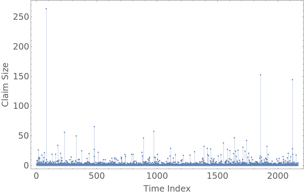
Plot the data:
| In[2]:= |
| Out[3]= |  |
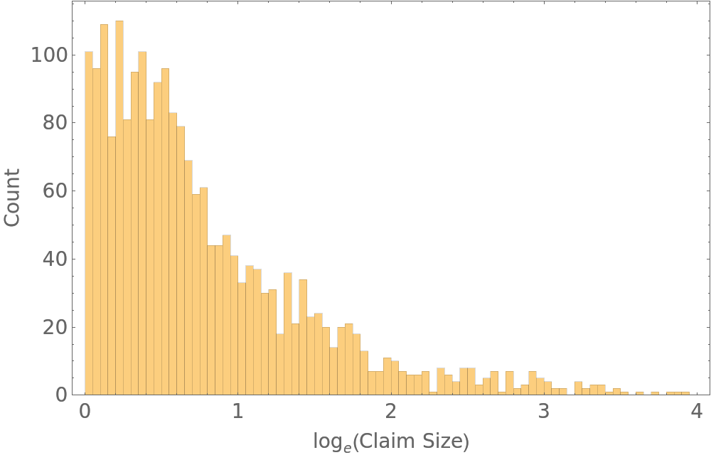
Construct a histogram of the log claim size:
| In[4]:= | ![ts = ResourceData["Danish Fire Insurance Claims"];
dataDanish = ts["Values"];
Histogram[
Log[dataDanish], Sequence[{0, 4, 0.05}, PlotRange -> All, Axes -> False, Frame -> True, FrameLabel -> {"\!\(\*SubscriptBox[\(log\), \(e\)]\)(Claim Size)", "Count"}, ImageSize -> 500, BaseStyle -> {FontSize -> 14}]]](https://www.wolframcloud.com/obj/resourcesystem/images/4de/4deb3a67-d305-41c5-aa63-3e5175b36a2d/15deddc088fa8c35.png) |
| Out[6]= |  |
Threshold the data and fit to a Pareto distribution:
| In[7]:= | ![u = 10.0;
ts = ResourceData["Danish Fire Insurance Claims"];
dataDanish = ts["Values"];
data = Sort@Select[dataDanish, # > u &];
Nd = Length[data];
Clear[k, \[Alpha], \[Mu]];
d = EstimatedDistribution[data, ParetoDistribution[k, \[Alpha], \[Mu]]]](https://www.wolframcloud.com/obj/resourcesystem/images/4de/4deb3a67-d305-41c5-aa63-3e5175b36a2d/220968a25a4e7d85.png) |
| Out[13]= |
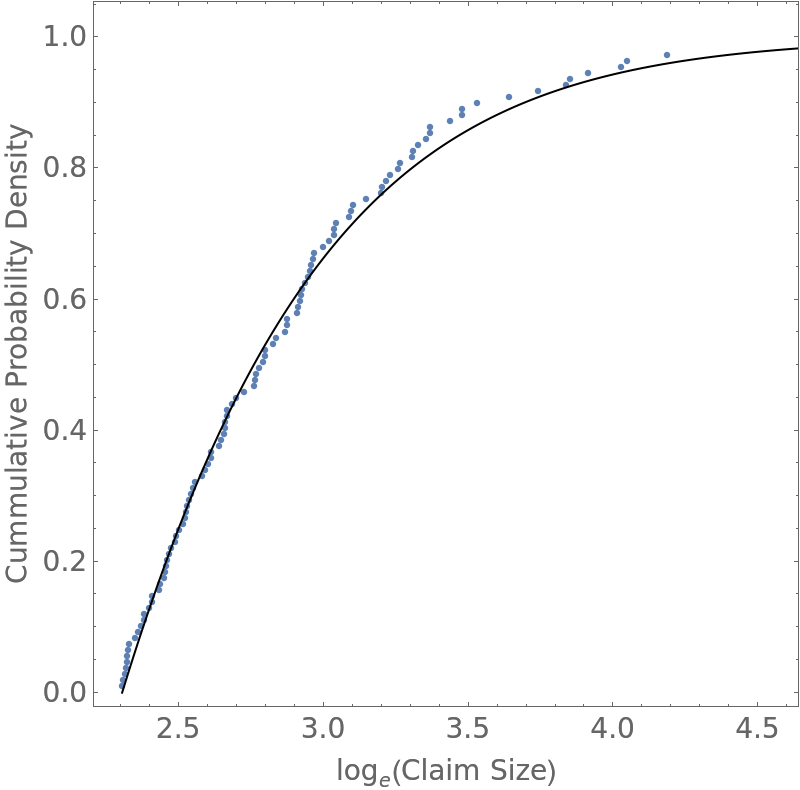
Compare empirical and theoretical cumulative probability distributions:
| In[14]:= | ![modelCDF = Table[{Log[x], CDF[d, x]}, {x, Min[data], Max[data], 0.1}];
empiricalCDF = Transpose[{Log[data], N@Table[n/Nd, {n, 1, Nd}]}];
ListPlot[empiricalCDF, Epilog -> {Line[modelCDF]}, Sequence[
Axes -> False, Frame -> True, FrameLabel -> {"\!\(\*SubscriptBox[\(log\), \(e\)]\)(Claim Size)", "Cummulative Probability Density"}, ImageSize -> 400, BaseStyle -> {FontSize -> 14}, AspectRatio -> 1]]](https://www.wolframcloud.com/obj/resourcesystem/images/4de/4deb3a67-d305-41c5-aa63-3e5175b36a2d/58d0d8c324f8188a.png) |
| Out[16]= |  |
Marshall Bradley, "Danish Fire Insurance Claims" from the Wolfram Data Repository (2022)