Locations of pine trees annotated with diameter (in centimeters) and height (in meters) marks
Examples
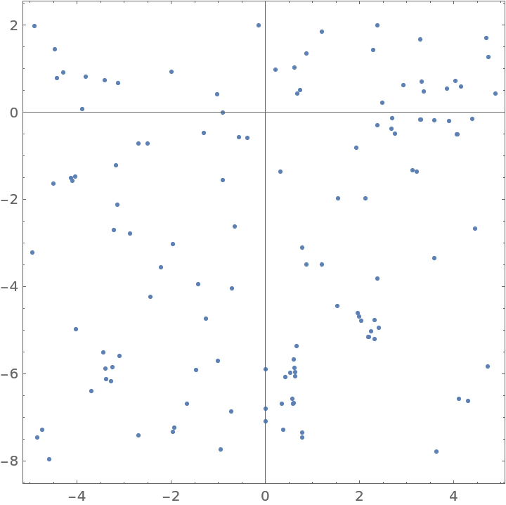
Basic Examples (1)
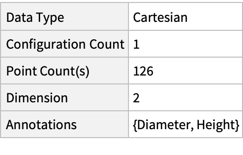
Summary of the spatial point data:
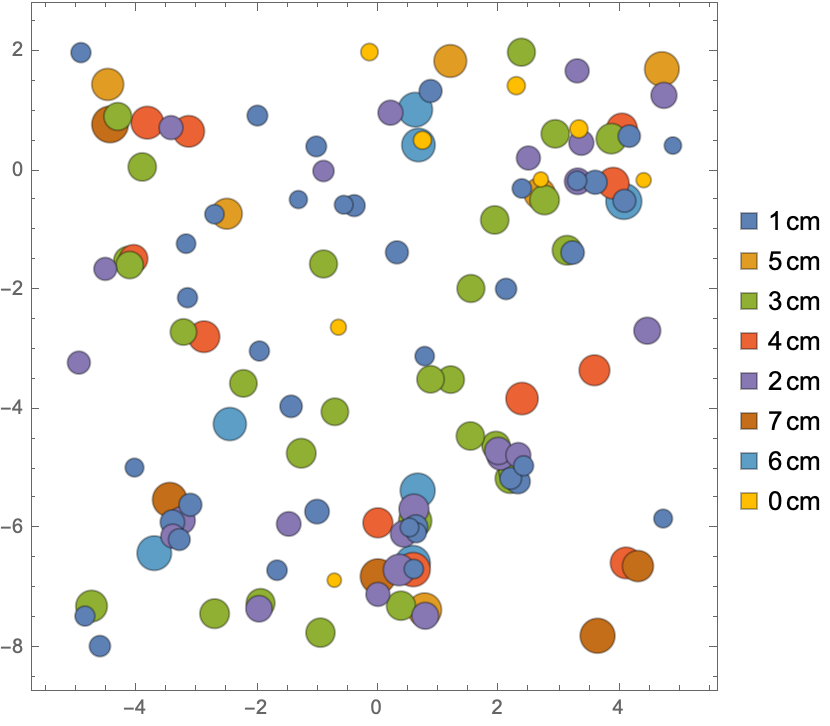
Visualizations (1)
Visualize points with diameter annotations:
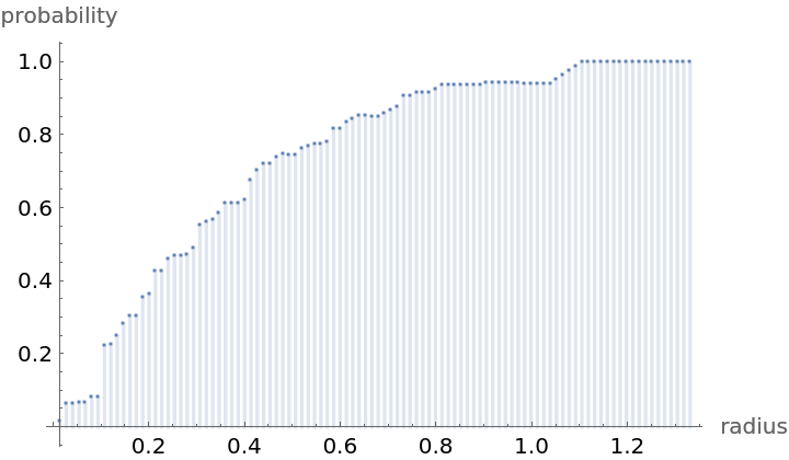
Analysis (5)
Compute probability of finding a point within given radius of an existing point - NearestNeighborG is the CDF of the nearest neighbor distribution:
NearestNeighborG as the CDF of nearest neighbor distribution can be used to compute the mean distance between a typical point and its nearest neighbor - the mean of a positive support distribution can be approximated via a Riemann sum of 1- CDF. To use Riemann approximation create the partition of the support interval from 0 to maxR into 100 parts and compute the value of the NearestNeighborG at the middle of each subinterval:
Now compute the Riemann sum to find the mean distance between a typical point and its nearest neighbor:
Test for complete spacial randomness:
Fit a Poisson point process to data:
Bibliographic Citation
Gosia Konwerska,
"Sample Data: Fin Pines"
from the Wolfram Data Repository
(2022)
Data Resource History
Publisher Information


![step = maxR/100;
middles = Subdivide[step/2, maxR - step/2, 99];
values = nnG[middles];](https://www.wolframcloud.com/obj/resourcesystem/images/1a9/1a9fd68b-58bf-43d9-a3cc-ef09e497b7ae/18a34a307439f124.png)