Details
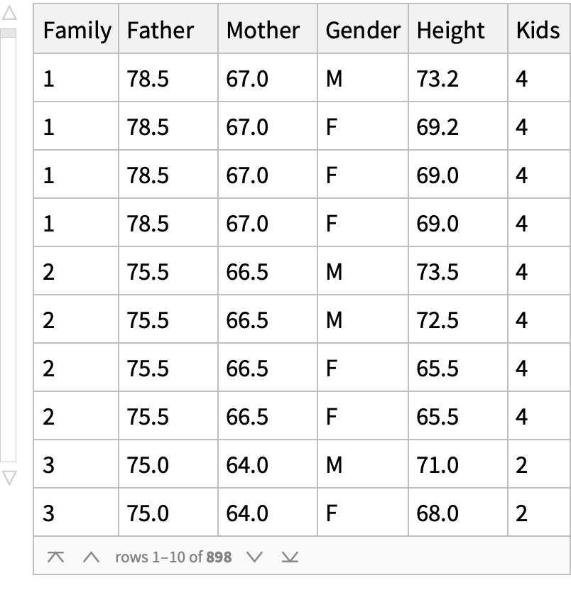
The data are due to Sir Francis Galton. The data set includes the following data for 205 families: The family that the child belongs to numbered from 1 to 205. The height of the father in inches. The height of the mother in inches. The gender of the child with male (M) or female (F). The height of the child in inches. The number of children in family of the child.
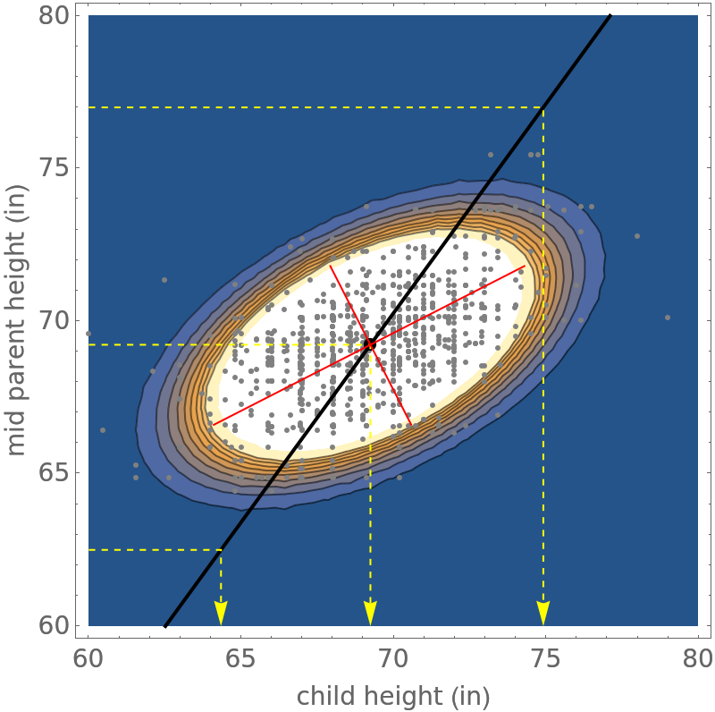
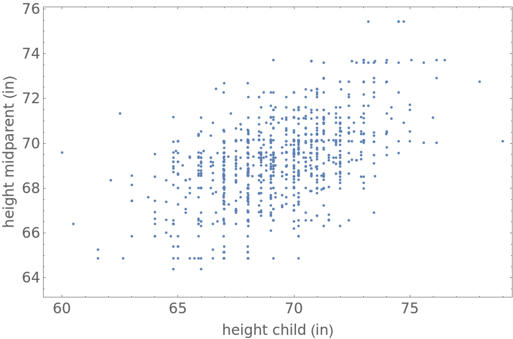
Galton reduced the analysis of the data to two variables by multiplying the female heights of the children by 1.08 and defining what he referred to as a midparent. The height of the midparent was defined to be hmid=(hfather+1.08hmother)/2. That is the midparent height is the average of the father's height and the mother's height adjusted by the factor 1.08. He then considered the distribution of the paired data (hi,ci) where hi is the height of the midparent and ci is the height of the adult child. He found that these data follow a binormal distribution with parameters {μc,μm,σc,σm,ρ) where μ denotes mean, σ denotes standard deviation and ρ is correlation coefficient. The probability density function of the joint distribution of child and midparent height is log p(h,c)∝(h-μh)2/σh2+(c-μc)2/σc2-2ρ(h-μh)(c-μc)/(σmσc). Thus the distribution is elliptical in shape with the tilt of the ellipse controlled by the correlation ρ.
Galton went on to investigate whether children of tall parents tend to be tall and what to degree. He found that children of tall parents tend to be taller than average but not as tall as their parents. Similarly children of shorter parents tend to be shorter than average but taller than their parents. This is referred to as regression to the mean and is necessary in order to maintain a stable distribution of population height.
The mean of the conditional distribution p(c|h=h0) is μc+(h0-μm)ρ σc/σm. If the midparent height in question h0 is equal to the mean of the midparent heights μm then the height of the child can be expect to equal to the mean μc of the children heights. However if the value of h0 is smaller than μm then the height of the child can be expected to be greater than the height of the midparent, but less than average in height. Correspondingly if the value of h0 is greater than μm then the height of the child can be expected to be less than the height of the midparent, but above average in height.
![father = Normal[resource[All, 2]]; mother = Normal[resource[All, 3]];
children = Transpose[Table[Normal[resource[All, i]], {i, {4, 5}}]];
maleAdultChild = Map[Last, Select[children, First[#] == "M" &]];
femaleAdultChild = Map[Last, Select[children, First[#] == "F" &]];
people = {father, mother, maleAdultChild, femaleAdultChild};
mean = Map[Mean, people]; sd = Map[StandardDeviation, people];
ns = Map[Length, people]; type = {"Father", "Mother", "Male child", "Female child"};
TableForm[Transpose[{mean, sd, ns}], TableHeadings -> {type, {"Mean", "Standard deviation", "Samples"}}]](https://www.wolframcloud.com/obj/resourcesystem/images/9fe/9fe3a98c-05e9-4633-b175-37facba21ebb/67106b82c604fca3.png)

![father = Normal[resource[All, 2]]; mother = Normal[resource[All, 3]];
\[Mu]F = Mean[father]; sF = StandardDeviation[father]; nF = Length[father];
\[Mu]M = Mean[mother]; sM = StandardDeviation[mother]; nM = Length[mother];
cdfF = Transpose[{Sort[father], Table[i/(nF + 1), {i, 1, nF}]}];
cdfM = Transpose[{Sort[mother], Table[i/(nM + 1), {i, 1, nM}]}];
min = Min[mother]; max = Max[father];
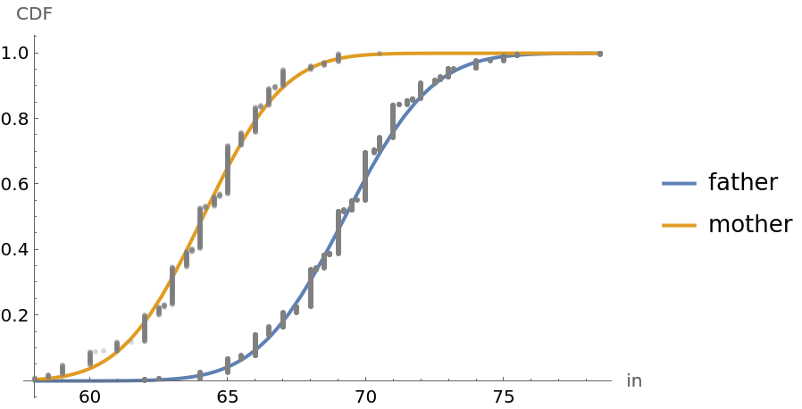
Plot[{CDF[NormalDistribution[\[Mu]F, sF], h], CDF[NormalDistribution[\[Mu]M, sM], h]}, {h, min, max}, Epilog -> {{Gray, Point[cdfF]}, {Opacity[0.3], Gray, Point[cdfM]}}, Sequence[
AxesLabel -> {"in", "CDF"}, PlotStyle -> {Thick, Thick}, PlotLegends -> {"father", "mother"}]]](https://www.wolframcloud.com/obj/resourcesystem/images/9fe/9fe3a98c-05e9-4633-b175-37facba21ebb/16d6cd60e94ededf.png)
![children = Transpose[Table[Normal[resource[All, i]], {i, {4, 5}}]];
mC = Map[Last, Select[children, First[#] == "M" &]];
fC = Map[Last, Select[children, First[#] == "F" &]];
\[Mu]mC = Mean[mC]; smC = StandardDeviation[mC]; nmC = Length[mC];
\[Mu]fC = Mean[fC]; sfC = StandardDeviation[fC]; nfC = Length[fC];
cdfmC = Transpose[{Sort[mC], Table[i/(nmC + 1), {i, 1, nmC}]}];
cdffC = Transpose[{Sort[fC], Table[i/(nfC + 1), {i, 1, nfC}]}];
min = Min[fC]; max = Max[mC];
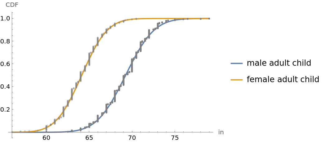
Plot[{CDF[NormalDistribution[\[Mu]mC, smC], h], CDF[NormalDistribution[\[Mu]fC, sfC], h]}, {h, min, max}, Epilog -> {{Gray, Point[cdfmC]}, {Opacity[0.3], Gray, Point[cdffC]}}, Sequence[
AxesLabel -> {"in", "CDF"}, PlotStyle -> {Thick, Thick}, PlotLegends -> {"male adult child", "female adult child"}]]](https://www.wolframcloud.com/obj/resourcesystem/images/9fe/9fe3a98c-05e9-4633-b175-37facba21ebb/515bafbf69ec1348.png)

![resource = ResourceData[\!\(\*
TagBox["\"\<Galton Parent and Child Height Data\>\"",
#& ,
BoxID -> "ResourceTag-Galton Parent and Child Height Data-Input",
AutoDelete->True]\)];
data = Table[
{f, m, g, h} = {"Father", "Mother", "Gender", "Height"} /. Normal[resource[[i]]];
mid = (f + 1.08 m)/2;
{If[g == "M", h, 1.08 h], mid}, {i, 1, Length[resource]}];
ListPlot[data, Sequence[
PlotRange -> All, Axes -> False, Frame -> True, PlotRange -> All, FrameLabel -> {"height child (in)", "height midparent (in)"}, ImageSize -> 500, BaseStyle -> {FontSize -> 14}]]](https://www.wolframcloud.com/obj/resourcesystem/images/9fe/9fe3a98c-05e9-4633-b175-37facba21ebb/75236f18560edd6f.png)
![{child, midparent} = Transpose[data]; Clear[a, b];
edc = EstimatedDistribution[child, NormalDistribution[a, b]];
edm = EstimatedDistribution[midparent, NormalDistribution[a, b]];
gc = Show[
Histogram[child, {60, 80, 1}, "PDF", PlotLabel -> "child", AxesLabel -> {"in"}], Plot[PDF[edc, x], {x, 60, 80}]];
gm = Show[
Histogram[midparent, {60, 80, 1}, "PDF", Sequence[
PlotLabel -> "midparent", AxesLabel -> {"in"}]], Plot[PDF[edm, x], {x, 60, 80}]];
GraphicsRow[{gm, gc}]](https://www.wolframcloud.com/obj/resourcesystem/images/9fe/9fe3a98c-05e9-4633-b175-37facba21ebb/48d953f9d15326c2.png)

![resource = ResourceData[\!\(\*
TagBox["\"\<Galton Parent and Child Height Data\>\"",
#& ,
BoxID -> "ResourceTag-Galton Parent and Child Height Data-Input",
AutoDelete->True]\)];
data = Table[
{f, m, g, h} = {"Father", "Mother", "Gender", "Height"} /. Normal[resource[[i]]];
mid = (f + 1.08 m)/2;
{If[g == "M", h, 1.08 h], mid}, {i, 1, Length[resource]}];
Clear[\[Mu]c, \[Mu]m, \[Sigma]c, \[Sigma]m, \[Rho], x, y, y0];
dist = EstimatedDistribution[data, BinormalDistribution[{\[Mu]c, \[Mu]m}, {\[Sigma]c, \[Sigma]m}, \[Rho]]];
{\[Mu]c, \[Mu]m} = dist[[1]]; {\[Sigma]c, \[Sigma]m} = dist[[2]]; \[Rho] = dist[[3]];
TableForm[{{\[Mu]c, \[Mu]m, \[Sigma]c, \[Sigma]m, \[Rho]}}, TableHeadings -> {None, {"\[Mu]c", "\[Mu]m", "\[Sigma]c", "\[Sigma]m", "\[Rho]"}}]](https://www.wolframcloud.com/obj/resourcesystem/images/9fe/9fe3a98c-05e9-4633-b175-37facba21ebb/1ed3956aa196b6b3.png)
![xmin = 60; xmax = 80; ymin = 60; ymax = 80;
mean = {PointSize[0.02], Point[{\[Mu]c, \[Mu]m}]}; datapoints = {Gray,
Point[data]};
reference = Table[pnt1 = {xmin, y0}; pnt2 = {\[Mu]c + ((y0 - \[Mu]m) \[Rho] \[Sigma]c)/\[Sigma]m, y0}; pnt3 = {\[Mu]c + ((y0 - \[Mu]m) \[Rho] \[Sigma]c)/\[Sigma]m, ymin};
ref = {Yellow, Dashing[0.01], Arrow[{pnt1, pnt2, pnt3}]}; ref, {y0, {62.5, \[Mu]m, 77}}];
conditional = {Black, Thick, Line[Table[{\[Mu]c + ((y0 - \[Mu]m) \[Rho] \[Sigma]c)/\[Sigma]m, y0}, {y0, ymin, ymax, 0.1}]]};
major = {Red, Line[Table[{\[Mu]c + (y0 - \[Mu]m)/\[Rho], y0}, {y0, 66.6, 71.85, 0.1}]]};
minor = {Red, Line[Table[{\[Mu]c - \[Rho] (y0 - \[Mu]m), y0}, {y0, 66.6, 71.85, 0.1}]]};
ContourPlot[PDF[dist, {x, y}], {x, xmin, xmax}, {y, ymin, ymax}, Epilog -> {datapoints, mean, conditional, reference, major, minor}, Sequence[
AspectRatio -> 1, FrameLabel -> {"child height (in)", "mid parent height (in)"}, ImageSize -> 400, BaseStyle -> {FontSize -> 14}]]](https://www.wolframcloud.com/obj/resourcesystem/images/9fe/9fe3a98c-05e9-4633-b175-37facba21ebb/7454d8d61c7bc9b6.png)