Geiger Counter Data

Counts of α-particles given by Rutherford and Geiger

Details

These data were used by Harold Jeffreys in his book Scientific Inference to illustrate properties of the Poisson probability distribution. The chi-square method was in turn used to give a quantitative standard of agreement between observation and theory. The actual Geiger counter data are in the first two columns of the data table. The first column gives the number of α-particles observed in an interval of time. The second column gives the number intervals when that number of particles were ejected. The total number of intervals in the data set is 2608. The total number of particles is 10097.

Jeffreys fitted these data to a Poisson distribution and obtained a mean value of the Poisson parameter of μ=3.87. The expected number of observations for m=0,1…14 particles in an interval is 2608 e^-μμ^m/m!. These expected values are tabulated in the 3rd column of the table and the difference between the observed values and expected values are given in the 4th column.

Individual chi-square values are given in the 5th column of the data table. In his analysis of the data Jeffreys lumped the data for 11 or more observations into a single observation with an observed minus expected value of +1 and an individual chi-square values of 0.2. Total Χ²=Σ(O-E)²/E=13.3.

(5 columns, 15 rows)

Examples

Basic Examples (2)

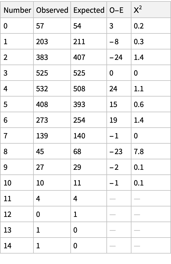
View the data table:

In[1]:=

$ResourceData[\!$\* TagBox["\"\<Geiger Counter Data\>\"", #& , BoxID -> "ResourceTag-Geiger Counter Data-Input", AutoDelete->True]$]$

Out[1]=

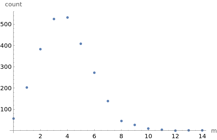
Plot the number of α-particles in an interval of time versus observed count. In the figure m is the number of α particles observed in a particular interval and count is the total number of times that number of particles was observed in the entire experiment:

In[2]:=

$dataset = ResourceData[\!$\* TagBox["\"\<Geiger Counter Data\>\"", #& , BoxID -> "ResourceTag-Geiger Counter Data-Input", AutoDelete->True]$]; number = Table[dataset[[i]][[1]], {i, 1, 15}]; observed = Table[dataset[[i]][[2]], {i, 1, 15}]; ListPlot[Transpose[{number, observed}], AxesLabel -> {"m", "count"}]$

Out[5]=

Scope & Additional Elements (3)

The mean of the data is:

In[6]:=

Out[9]=

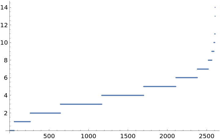
The observations from which the first two columns of the data table were constructed are:

In[10]:=

Out[11]=

The mean can also be calculated from these:

In[12]:=

Out[12]=

Visualizations (3)

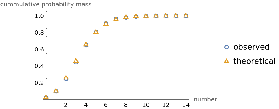
In the following we compute the empirical cumulative mass function and compare it to the theoretical cumulative probability mass function. The first is to find the mean of the observed data:

In[13]:=

$dataset = Dataset[ResourceData[\!$\* TagBox["\"\<Geiger Counter Data\>\"", #& , BoxID -> "ResourceTag-Geiger Counter Data-Input", AutoDelete->True]$]]; number = Table[dataset[[i]][[1]], {i, 1, 15}]; observed = Table[dataset[[i]][[2]], {i, 1, 15}]; \[Mu] = N@number . observed/Total[observed]$

Out[2]=

The empirical probability mass function is:

In[14]:=

The comparison between observed and theoretical probability mass functions is:

In[15]:=

$cdfobs = Table[{i, cdf[i]}, {i, 0, 14}]; cdftheo = Table[{i, CDF[PoissonDistribution[\[Mu]], i]}, {i, 0, 14}]; ListPlot[{cdfobs, cdftheo}, Sequence[ AxesLabel -> {"number", "cummulative probability mass"}, PlotLegends -> {"observed", "theoretical"}, PlotMarkers -> "OpenMarkers"]]$

Out[6]=

Analysis (6)

Key data quantities are imported here:

In[16]:=

$dataset = ResourceData[\!$\* TagBox["\"\<Geiger Counter Data\>\"", #& , BoxID -> "ResourceTag-Geiger Counter Data-Input", AutoDelete->True]$]; observed = Table[dataset[[i]][[2]], {i, 1, 15}];$

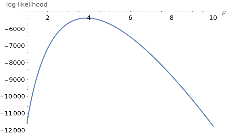
The log likelihood of the observed data as a function of the Poisson parameter μ is:

In[17]:=

$logLikelihood[\[Mu]_] := Sum[observed[[m + 1]] (m*Log[\[Mu]] - \[Mu] - Log[Factorial[m]]), {m, 0, 14}] Plot[logLikelihood[\[Mu]], {\[Mu], 1, 10}, AxesLabel -> {"\[Mu]", "log likelihood"}]$

Out[2]=

The values of μ that maximizes the log likelihood is:

In[18]:=

$Clear[\[Mu]]; FindMaximum[logLikelihood[\[Mu]], {\[Mu], 3}]$

Out[15]=

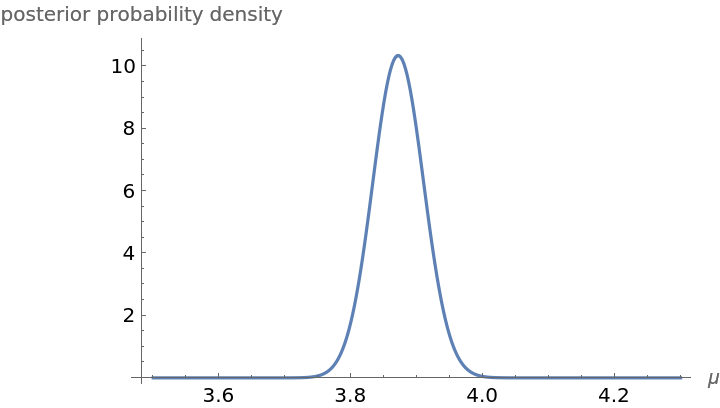
The Bayesian posterior probability distribution for μ on the assumption of a flat prior for μ on the interval (3.5,4.3) is:

In[19]:=

$\[Mu]min = 3.5; \[Mu]max = 4.3; d\[Mu] = 0.0025; logpdf = Table[logLikelihood[\[Mu]], {\[Mu], \[Mu]min, \[Mu]max, d\[Mu]}]; logpdf = logpdf - Max[logpdf]; pdf = Exp[logpdf]; pdf = (d\[Mu]^-1) pdf/Total[pdf]; ListLinePlot[pdf, Sequence[ PlotRange -> All, DataRange -> {\[Mu]min, \[Mu]max}, AxesLabel -> {"\[Mu]", "posterior probability density"}]]$