Wolfram Research

Sample Data: Hyytiala Trees

Source Notebook

Locations of trees recorded at Hyytiala, Finland, annotated with species (pine/birch/rowan/aspen) marks

Details

Locations of trees recorded at Hyytiala, Finland, in the observation region Rectangle[{0., 0.}, {20., 20.}] meters, annotated with species (pine / birch / rowan / aspen) marks.

Examples

Basic Examples (1) 

In[1]:=
ResourceData[\!\(\*
TagBox["\"\<Sample Data: Hyytiala Trees\>\"",
#& ,
BoxID -> "ResourceTag-Sample Data: Hyytiala Trees-Input",
AutoDelete->True]\), "Data"]
Out[1]=

Summary of the spatial point data:

In[2]:=
ResourceData[\!\(\*
TagBox["\"\<Sample Data: Hyytiala Trees\>\"",
#& ,
BoxID -> "ResourceTag-Sample Data: Hyytiala Trees-Input",
AutoDelete->True]\), "Data"]["Summary"]
Out[2]=

Visualizations (2) 

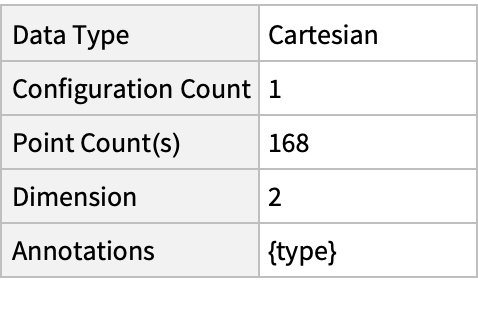
Plot the spatial point data:

In[3]:=
ListPlot[ResourceData[\!\(\*
TagBox["\"\<Sample Data: Hyytiala Trees\>\"",
#& ,
BoxID -> "ResourceTag-Sample Data: Hyytiala Trees-Input",
AutoDelete->True]\), "Data"]]
Out[3]=

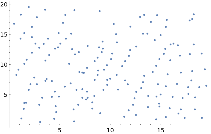
Visualize tree locations with type annotations:

In[4]:=
PointValuePlot[ResourceData[\!\(\*
TagBox["\"\<Sample Data: Hyytiala Trees\>\"",
#& ,
BoxID -> "ResourceTag-Sample Data: Hyytiala Trees-Input",
AutoDelete->True]\), "Data"], PlotLegends -> Automatic]
Out[4]=

Analysis (6) 

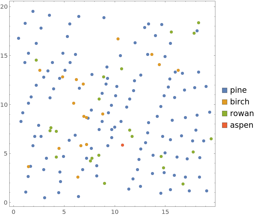
Compute probability of finding a point within given radius of an existing point - NearestNeighborG is the CDF of the nearest neighbor distribution:

In[5]:=
nnG = NearestNeighborG[ResourceData[\!\(\*
TagBox["\"\<Sample Data: Hyytiala Trees\>\"",
#& ,
BoxID -> "ResourceTag-Sample Data: Hyytiala Trees-Input",
AutoDelete->True]\), "Data"]]
Out[5]=
In[6]:=
maxR = nnG["MaxRadius"]
Out[6]=
In[7]:=
DiscretePlot[nnG[r], {r, maxR/100, maxR, maxR/100}, AxesLabel -> {"radius", "probability"}]
Out[7]=

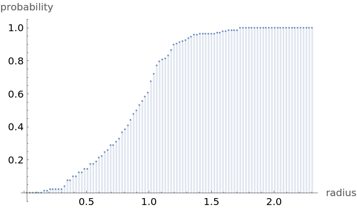
NearestNeighborG as the CDF of nearest neighbor distribution can be used to compute the mean distance between a typical point and its nearest neighbor - the mean of a positive support distribution can be approximated via a Riemann sum of 1- CDF. To use Riemann approximation create the partition of the support interval from 0 to maxR into 100 parts and compute the value of the NearestNeighborG at the middle of each subinterval:

In[8]:=
step = maxR/100;
middles = Subdivide[step/2, maxR - step/2, 99];
values = nnG[middles];

Now compute the Riemann sum to find the mean distance between a typical point and its nearest neighbor:

In[9]:=
Total[(1 - values)*step]
Out[9]=

In region units:

In[10]:=
%*ResourceData[\!\(\*
TagBox["\"\<Sample Data: Hyytiala Trees\>\"",
#& ,
BoxID -> "ResourceTag-Sample Data: Hyytiala Trees-Input",
AutoDelete->True]\), "RegionScale"]
Out[10]=

Test for complete spacial randomness:

In[11]:=
SpatialRandomnessTest[ResourceData[\!\(\*
TagBox["\"\<Sample Data: Hyytiala Trees\>\"",
#& ,
BoxID -> "ResourceTag-Sample Data: Hyytiala Trees-Input",
AutoDelete->True]\), "Data"], {"PValue", "TestConclusion"}]
Out[11]=

Fit a Poisson point process to data:

In[12]:=
EstimatedPointProcess[ResourceData[\!\(\*
TagBox["\"\<Sample Data: Hyytiala Trees\>\"",
#& ,
BoxID -> "ResourceTag-Sample Data: Hyytiala Trees-Input",
AutoDelete->True]\), "Data"], PoissonPointProcess[\[Mu], 2]]
Out[12]=

Gosia Konwerska, "Sample Data: Hyytiala Trees" from the Wolfram Data Repository (2022)  

Data Resource History

Source Metadata

Publisher Information