Wolfram Data Repository
Immediate Computable Access to Curated Contributed Data
Relationship between the mass of a black hole and galaxy bulge velocity dispersion
(4 columns, 31 rows)
| In[1]:= |
| Out[1]= | 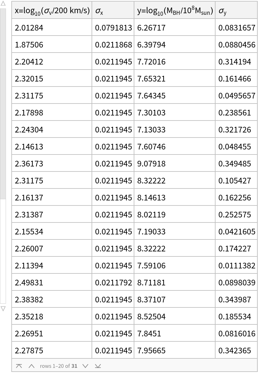 |
Organize the data in a matrix format and display the first 9 rows:
| In[2]:= | ![observedX = Normal@xydata[All, 1];
observedErrorX = Normal@xydata[All, 2];
observedY = Normal@xydata[All, 3];
observedErrorY = Normal@xydata[All, 4];
Transpose[{observedX, observedErrorX, observedY, observedErrorY}];
MatrixForm[Take[%, {1, 9}]]](https://www.wolframcloud.com/obj/resourcesystem/images/5a3/5a3f724a-99f7-4927-a0e7-9b4ffa1d19a6/325d113b6b7c8f8d.png) |
| Out[7]= |  |
A plot of the data with error bars is:
| In[8]:= | ![xydata = ResourceData[\!\(\*
TagBox["\"\<Magorrian Relation in Astrophysics\>\"",
#& ,
BoxID -> "ResourceTag-Magorrian Relation in Astrophysics-Input",
AutoDelete->True]\)];
observedX = Normal@xydata[All, 1];
observedErrorX = Normal@xydata[All, 2];
observedY = Normal@xydata[All, 3];
observedErrorY = Normal@xydata[All, 4];
pntsLeftX = Transpose[{observedX - observedErrorX, observedY}];
pntsRightX = Transpose[{observedX + observedErrorX, observedY}];
pntsUpY = Transpose[{observedX, observedY + observedErrorY}];
pntsDownY = Transpose[{observedX, observedY - observedErrorY}];
errorLines = Join[Transpose[{pntsLeftX, pntsRightX}], Transpose[{pntsDownY, pntsUpY}] ];
errorLines = {Black, Thin, Map[Line, errorLines]};
ListPlot[Transpose[{observedX, observedY}] , Prolog -> {errorLines} , Sequence[PlotStyle -> {
PointSize[0.02]}, PlotRange -> {{1.7, 2.7}, {6, 10}}, FrameLabel -> {"\!\(\*SubscriptBox[\(log\), \(10\)]\)(\!\(\*SubscriptBox[\(\[Sigma]\), \(v\)]\)/200 km/s)", "\!\(\*SubscriptBox[\(log\), \(10\)]\)(\!\(\*SubscriptBox[\(M\), \(BH\)]\)/ \!\(\*SuperscriptBox[\(10\), \(8\)]\)\!\(\*SubscriptBox[\(M\), \(sun\)]\))"}, BaseStyle -> {FontFamily -> "Arial", FontSize -> 14}, Axes -> False,
Frame -> True, ImageSize -> 400, AspectRatio -> 1, PlotRange -> All]]](https://www.wolframcloud.com/obj/resourcesystem/images/5a3/5a3f724a-99f7-4927-a0e7-9b4ffa1d19a6/1316303205fd52ca.png) |
| Out[12]= | 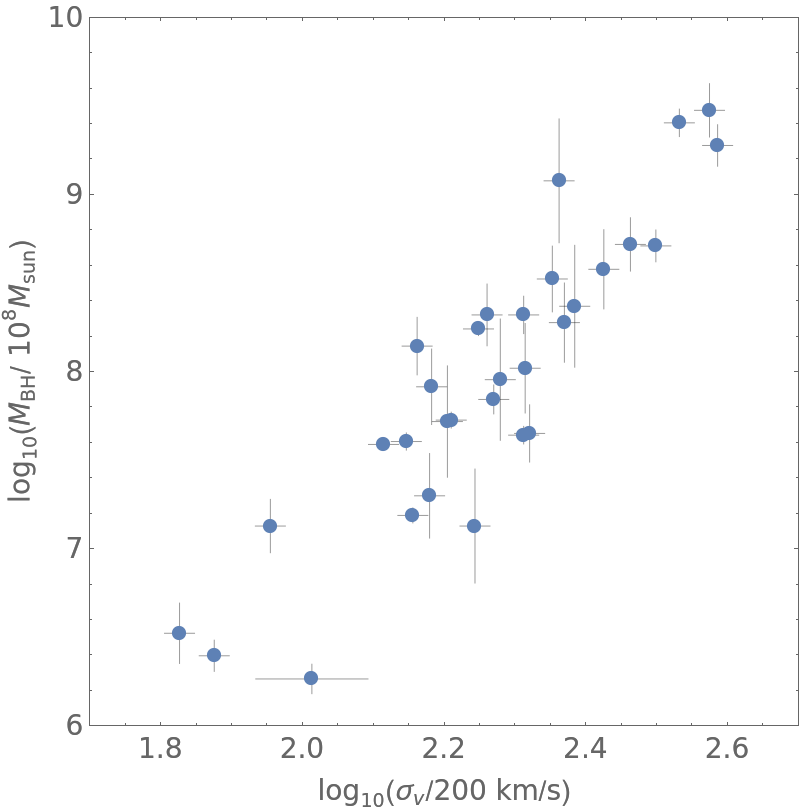 |
We start by acquiring the data that we need:
| In[13]:= | ![xydata = ResourceData[\!\(\*
TagBox["\"\<Magorrian Relation in Astrophysics\>\"",
#& ,
BoxID -> "ResourceTag-Magorrian Relation in Astrophysics-Input",
AutoDelete->True]\)];
observedX = Normal@xydata[All, 1];
observedErrorX = Normal@xydata[All, 2];
observedY = Normal@xydata[All, 3];
observedErrorY = Normal@xydata[All, 4];](https://www.wolframcloud.com/obj/resourcesystem/images/5a3/5a3f724a-99f7-4927-a0e7-9b4ffa1d19a6/1f7bca0a8d3cb1f2.png) |
In mathematical terms the likelihood of all n data pairs (xi,yi) and their respective standard deviations (σx,i,σy,i) is as follows:

In this expression a is the slope of the best fit line, b is the intercept of the line and σ is the intrinsic dispersion.
The following block of code computes the log likelihood of the data. Computations are performed on a log scale to avoid underflow and overflow:
| In[14]:= | ![Clear[logLikelihood, a, b, \[Sigma]];
logLikelihood[a_, b_, \[Sigma]_] := Module[{x, \[Sigma]x, y, \[Sigma]y, logL},
x = observedX; \[Sigma]x = observedErrorX;
y = observedY; \[Sigma]y = observedErrorY;
logL = -Length[x] Log[Sqrt[2.0 \[Pi]]] + Sum[-0.5 (y[[i]] - a*x[[i]] - b)^2/(\[Sigma]^2 + a^2 \[Sigma]x[[i]]^2 + \[Sigma]y[[i]]^2)
- Log[
Sqrt[\[Sigma]^2 + a^2 \[Sigma]x[[i]]^2 + \[Sigma]y[[i]]^2]], {i, 1, Length[x]}];
logL]](https://www.wolframcloud.com/obj/resourcesystem/images/5a3/5a3f724a-99f7-4927-a0e7-9b4ffa1d19a6/4df46e8276db2f78.png) |
The best fit parameters are in terms of maximum likelihood are:
| In[15]:= | ![Clear[a, b, \[Sigma]];
sol = Quiet@
FindMaximum[{logLikelihood[a, b, \[Sigma]], \[Sigma] > 0}, {a, 3.0}, {b, -1.0}, {\[Sigma], 0.3}];
{aML, bML, \[Sigma]ML} = {a, b, \[Sigma]} /. sol[[2]]](https://www.wolframcloud.com/obj/resourcesystem/images/5a3/5a3f724a-99f7-4927-a0e7-9b4ffa1d19a6/3976747b3c2a5366.png) |
| Out[17]= |
PLot the best fit line on the data:
| In[18]:= | ![bestFit = {Black, Thick, Line[Table[{x, aML*x + bML}, {x, 1.7, 2.7, 0.1}]]};
pntsLeftX = Transpose[{observedX - observedErrorX, observedY}];
pntsRightX = Transpose[{observedX + observedErrorX, observedY}];
pntsUpY = Transpose[{observedX, observedY + observedErrorY}];
pntsDownY = Transpose[{observedX, observedY - observedErrorY}];
errorLines = Join[Transpose[{pntsLeftX, pntsRightX}], Transpose[{pntsDownY, pntsUpY}] ];
errorLines = {Black, Thin, Map[Line, errorLines]};
ListPlot[Transpose[{observedX, observedY}] , Prolog -> {errorLines, bestFit} , Sequence[PlotStyle -> {
PointSize[0.02]}, PlotRange -> {{1.7, 2.7}, {6, 10}}, FrameLabel -> {"\!\(\*SubscriptBox[\(log\), \(10\)]\)(\!\(\*SubscriptBox[\(\[Sigma]\), \(v\)]\)/200 km/s)", "\!\(\*SubscriptBox[\(log\), \(10\)]\)(\!\(\*SubscriptBox[\(M\), \(BH\)]\)/ \!\(\*SuperscriptBox[\(10\), \(8\)]\)\!\(\*SubscriptBox[\(M\), \(sun\)]\))"}, BaseStyle -> {FontFamily -> "Arial", FontSize -> 14}, Axes -> False,
Frame -> True, ImageSize -> 400, AspectRatio -> 1, PlotRange -> All]]](https://www.wolframcloud.com/obj/resourcesystem/images/5a3/5a3f724a-99f7-4927-a0e7-9b4ffa1d19a6/42af93e6b9657cec.png) |
| Out[25]= | 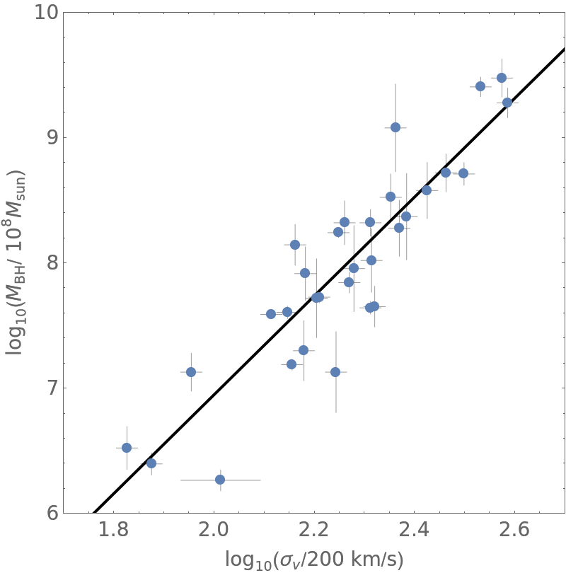 |
Marshall Bradley, "Magorrian Relation in Astrophysics" from the Wolfram Data Repository (2022)