Negative Binomial Distributed Accident Data

Number of accidents experienced by employees in a factory in a year

Details

These data do not follow a Poisson distribution but rather a negative binomial distribution. The reasoning is as follows. Careful people have few accidents and careless people have many accidents. The careless people give the distribution a long tail to the right. The careful people produce large numbers of either zero or one accidents. The combination of these two effects produces data which is a good fit to the negative binomial distribution.

(2 columns, 21 rows)

Examples

Basic Examples (2)

Display the ResourceObject data:

In[1]:=

$ResourceData[\!$\* TagBox["\"\<Negative Binomial Distributed Accident Data\>\"", #& , BoxID -> "ResourceTag-Negative Binomial Distributed Accident Data-Input", AutoDelete->True]$]$

Out[1]=

Plot the accident data:

In[2]:=

$dataset = ResourceData[\!$\* TagBox["\"\<Negative Binomial Distributed Accident Data\>\"", #& , BoxID -> "ResourceTag-Negative Binomial Distributed Accident Data-Input", AutoDelete->True]$]; number = Table[dataset[[i]][[1]], {i, 1, 21}]; observed = Table[dataset[[i]][[2]], {i, 1, 21}]; ListPlot[Transpose[{number, observed}], AxesLabel -> {"accidents", "count"}]$

Out[5]=

Visualizations (1)

Compare the observed data to fits to the Poisson and negative binomial distributions. The negative binomial fit is much better:

In[6]:=

$dataset = Dataset[ResourceData[\!$\* TagBox["\"\<Negative Binomial Distributed Accident Data\>\"", #& , BoxID -> "ResourceTag-Negative Binomial Distributed Accident Data-Input", AutoDelete->True]$]]; observed = Table[dataset[[i]][[2]], {i, 1, 21}]; observations = Flatten@Table[Table[i - 1, {observed[[i]]}], {i, 1, 21}]; Clear[\[Mu], r, p]; distPoisson = EstimatedDistribution[observations, PoissonDistribution[\[Mu]]]; distNB = EstimatedDistribution[observations, NegativeBinomialDistribution[r, p]]; empiricalPDF = N@Transpose[{number, observed/Total[observed]}]; theoPoisson = Table[{r, PDF[distPoisson, r]}, {r, 0, 20, 1}]; theoNB = Table[{r, PDF[distNB, r]}, {r, 0, 20, 1}]; ListPlot[{empiricalPDF, theoPoisson, theoNB}, Sequence[ PlotLegends -> {"observed", "Poisson", "Negative Binomial"}, PlotMarkers -> {Automatic, Medium}, Joined -> {False, False, True}, AxesLabel -> {"accidents", "probability mass"}]]$

Out[7]=

Analysis (10)

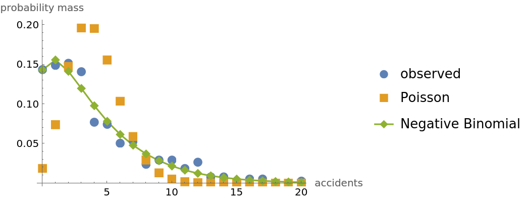
The focus here is on comparing the Poisson fit to the negative binomial fit. Goodness of fit is measured via a comparison of the Bayesian evidence favoring each of the two models.

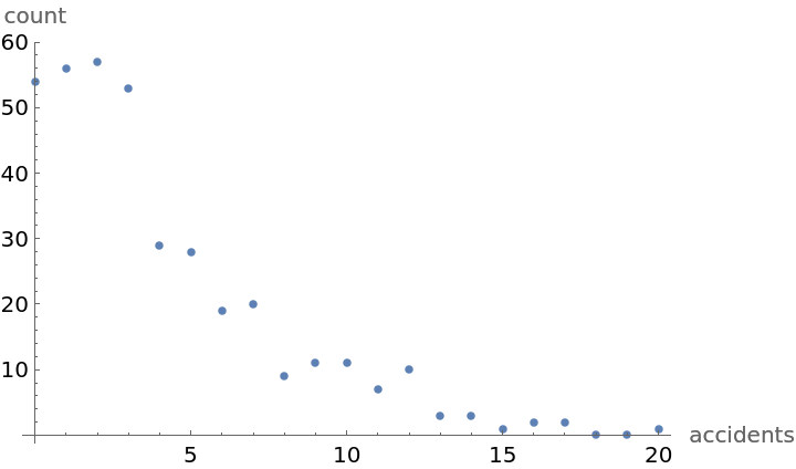
Read in the data and find the mean:

In[8]:=

Out[9]=

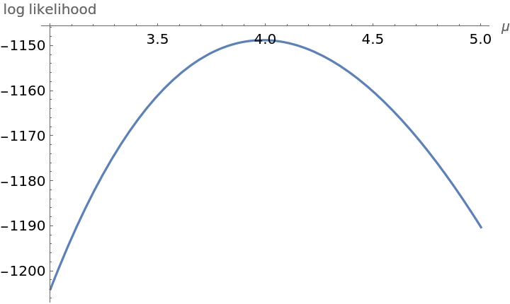
The Poisson random variable has one parameter namely the mean μ. Plot the log likelihood of the data under the assumption that it is Poisson distributed:

In[10]:=

$Clear[\[Mu]]; logLikelihoodPoisson[\[Mu]_] := N@Sum[observed[[ m + 1]] (m*Log[\[Mu]] - \[Mu] - Log[Factorial[m]]), {m, 0, 20}] Plot[logLikelihoodPoisson[\[Mu]], {\[Mu], 3.0, 5.0}, AxesLabel -> {"\[Mu]", "log likelihood"}]$

Out[11]=

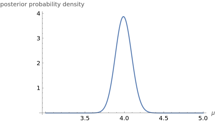
Plot the posterior probability density function for the parameter μ under the assumption that the prior probability distribution for μ is flat on the interval (μ_min,μ_max). Bayes theorem tell us that the posterior probability distribution is proportional to the product of the prior and the likelihood. The constant of proportionality known as the evidence and is found by numerical integration. Computations are performed on a log scale to avoid numerical underflow:

In[12]:=

$\[Mu]min = 3.0; \[Mu]max = 5.0; d\[Mu] = 0.0025; logpdf = Table[Log[1/(\[Mu]max - \[Mu]min)] + logLikelihoodPoisson[\[Mu]], {\[Mu], \[Mu]min, \[Mu]max, d\[Mu]}]; maxlog = Max[logpdf]; logpdf = logpdf - maxlog; pdf = Exp[logpdf]; pdf = (d\[Mu]^-1) pdf/Total[pdf]; ListLinePlot[pdf, Sequence[ PlotRange -> All, DataRange -> {\[Mu]min, \[Mu]max}, AxesLabel -> {"\[Mu]", "posterior probability density"}]]$

Out[17]=

Compute the Bayesian evidence in favor of the Poisson model:

In[18]:=

$\[Mu]min = 3.0; \[Mu]max = 5.0; d\[Mu] = 0.0025; logpdf = Table[Log[1/(\[Mu]max - \[Mu]min)] + logLikelihoodPoisson[\[Mu]], {\[Mu], \[Mu]min, \[Mu]max, d\[Mu]}]; maxlog = Max[logpdf]; logpdf = logpdf - maxlog; posterior = Exp[logpdf]; logEvidencePoisson = Log[d\[Mu]*Total[posterior]] + maxlog$

Out[22]=

The Bayesian evidence is only meaningful when compared to another model using the exact same data.

Now we turn our attention to the evidence computation of the negative binomial assumption. The negative binomial distribution has two unknown parameters r and p. The log likelihood of the data under the assumption of the negative binomial distribution is:

In[23]:=

$logLikelihoodNB[r_, p_] := N@Sum[observed[[ m + 1]] (m*Log[1 - p] + r*Log[p] + Log[Binomial[-1 + m + r, -1 + r]]), {m, 0, 20}]$

The evidence computation requires an integration over two dimensions. We assume that on prior information r is flat distributed on (0.1,5.0) and that p is flat distributed on (0.05,0.5). The results of the evidence computation are:

In[24]:=

rmin = 0.1; rmax = 5.0; nr = 201;
pmin = 0.05; pmax = 0.5; np = 151;
dr = (rmax - rmin)/(nr - 1); dp = (pmax - pmin)/(np - 1);
loggrid2d = Table[Log[1/(rmax - rmin) 1/(pmax - pmin)] + logLikelihoodNB[r, p], {r, rmin, rmax, dr}, {p, pmin, pmax, dp}];
maxlog = Max[Flatten[loggrid2d]];
loggrid2d = ArrayReshape[Flatten[loggrid2d] - maxlog, Dimensions[loggrid2d]];
logEvidenceNB = maxlog + Log[dp*dr*Total[Exp[Flatten[loggrid2d]]]]

Out[30]=

As a check compute the evidence using the function NItegrate:

In[31]:=

loggrid = Table[logLikelihoodNB[r, p], {r, rmin, rmax, dr}, {p, pmin, pmax, dp}];
lmax = Max[loggrid];
Quiet[NIntegrate[
1/(rmax - rmin) 1/(pmax - pmin) Exp[
logLikelihoodNB[r, p] - lmax], {r, rmin, rmax}, {p, pmin, pmax}]];
Log[%] + lmax

Out[34]=

The difference between the evidence in favor of the negative binomial model and the Poisson model is huge. The observed data clearly favor the negative binomial model relative to the Poisson model:

In[35]:=

Out[35]=

All the information in a Bayesian analysis is in the posterior. The posterior marginal probability density function for the parameters r and p are:

In[36]:=

posteriorPDF = Exp[loggrid2d];
posteriorPDF = 1/(dp*dr) (posteriorPDF/Total[Flatten[posteriorPDF]]);
pdfr = dp*Chop@Map[Total, Map[Flatten, posteriorPDF]];
pdfp = dr*Chop@Map[Total, Map[Flatten, Transpose[posteriorPDF]]];
gr = ListLinePlot[pdfr, DataRange -> {rmin, rmax}, PlotRange -> All, AxesLabel -> {"r", "probability density"}];
gp = ListLinePlot[pdfp, DataRange -> {pmin, pmax}, PlotRange -> All, AxesLabel -> {"p", "probability density"}];
GraphicsRow[{gr, gp}]

Out[42]=

These two marginal probability density functions are clearly consistent with results from the function EstimatedDistribution:

In[43]:=

Out[44]=

Bibliographic Citation

Marshall Bradley, "Negative Binomial Distributed Accident Data" from the Wolfram Data Repository (2022)

Data Resource History

Date Created: 14 October 2022

Source Metadata

Citation:
- Jeffreys, Sir Harold (1973), Scientific Inference, Cambridge University Press.

Publisher Information

Prepared for the Wolfram Data Repository By: Marshall Bradley
Publisher of Record: Marshall Bradley