Analysis (12)
Wind velocity inversion is the process through which the wind velocity profile (vx(z),vy(z),vz(z)) at altitude z is estimated from scalar Doppler velocity measurements made on WiPPR radar beams pointed in the cardinal directions (N, E, S, W). If all scattering objects were moving horizontally then sophisticated procedures would not be required to determine wind velocity from Doppler velocity, but this is not the case. Falling hydrometers and updrafts are common in the convective boundary layer. The first step in the inversion process is to form a data catalog. The following code extracts all echo contacts with more than a specified amount of signal-to-noise(SNR) ratio and organizes the contacts in a catalog(table) with the structure: (altitude, file number, Doppler velocity, cosX, cosY, cosZ, beam number). The radar beam pointing direction of the echo in a catalog entry is (cosX, cosY, cosZ).
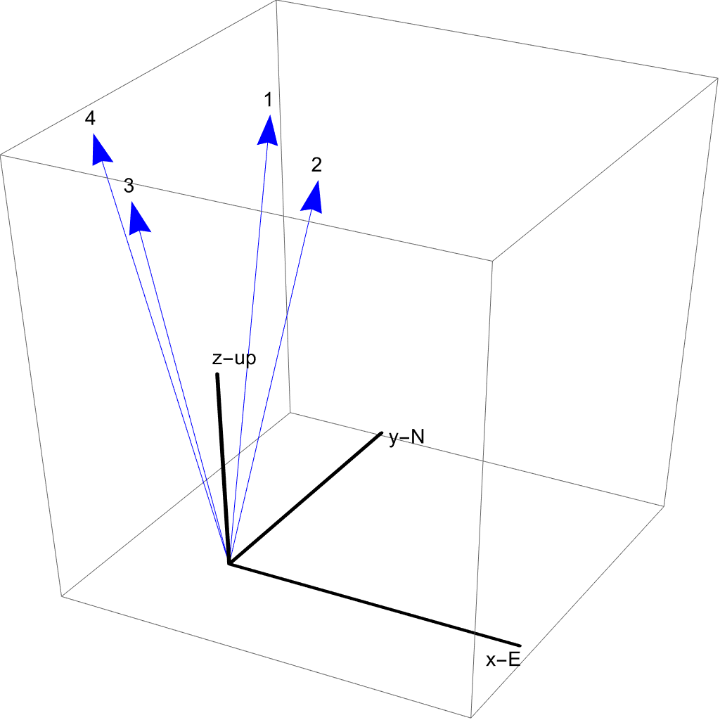
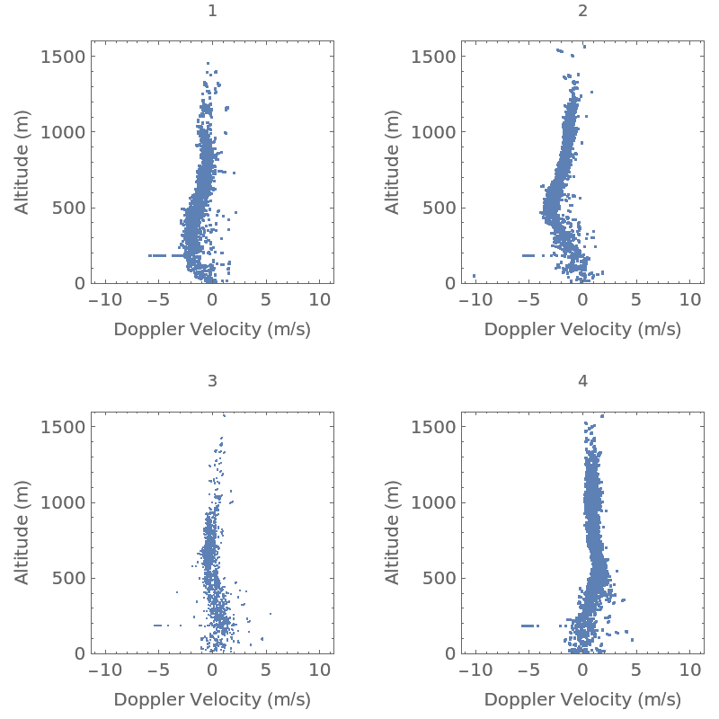
The following code constructs the WiPPR Doppler contact catalog:The catalog is calculated here:A small portion of the contact catalog is:Beams 1-4 are respectively pointed in the directions 1) north (0 deg), 2) east (90 deg), 3) south (180 deg) and 4) west (270 deg). The beams are nearly vertical with each beam elevated 80 deg from the horizontal, 10 deg off vertical. Provided that there is no vertical wind motion beam 3 directly measures the component of wind velocity component vy within the scale factor 1/cosθ where θ=80 deg. Beam 1 measures -vy within the scale factor. Beam 4 directly measures the vxcomponent of wind velocity within this scale factor. Beam 2 measures -vx within the scale factor.
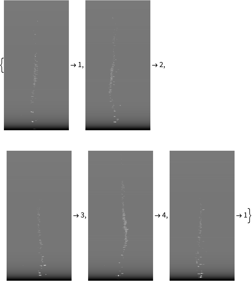
The following block of code groups the catalog contents by beam and makes a quad plot of the beam Doppler data:When executed the result is:Note the 180 deg left-right symmetry in the data between beam 1 and 3 and also between beams 2 and 4. This provides a strong indication that the WiPPR system was correctly functioning.
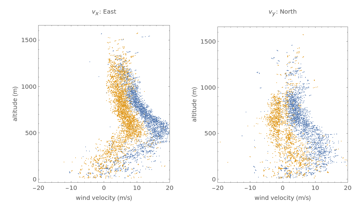
The following code computes the data necessary for a visual estimation of (vx,vy) that exploits the symmetry in the WiPPR beam geometry. The possible effect of falling hydrometers or a vertical component of the wind is ignored in this computation but is considered later:When executed the result is:There is an obvious offset between the beam 4 data and the reversed beam 2 data, see left figure. There is also an offset between the beam 3 data and the reversed beam 1 data, see right figure. These offsets are caused by non-zero vertical winds.
The relationship between wind velocity  and the observed Doppler velocity V is

where θ is the beam elevation angle and ϕ is the beam azimuth angle. If vz≠0 then the Doppler velocity will contain a contribution -vzsinθ. This complicates the velocity inversion process.
All the information necessary for a more refined estimate of the wind velocity profile (vx(z),vy(x),vz(z)) is in the data catalog. Suppose that at an altitude of interest the observed Doppler velocities are arranged into the vector  . The forward relationship between and the wind velocity is
  where A is the matrix of beam pointing directions corresponding to the entries in . Specifically, they are the data from columns 4-6 of the data catalog. Provided that A contains data from at least 3 unique beam pointing directions, then the least squares solution for the wind velocity is
 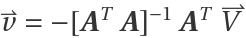 . In general it is best to require data from all four beams at an altitude before estimating the wind velocity vector. This reduces biasing effects. If θ is the beam elevation angle (80 deg for WiPPR) and ϕ the beam azimuthal angle, then the rows of the matrix A are of the form
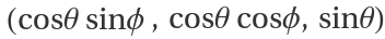 .
.
In the case where there are exactly four Doppler velocity measurements (V1,V2,V3,V4) at an altitude on beams (1,2,3,4) respectively then the least squares solution for the wind velocity (vx,vy,vz) takes a very simple form

where θ is the radar beam elevation angle.
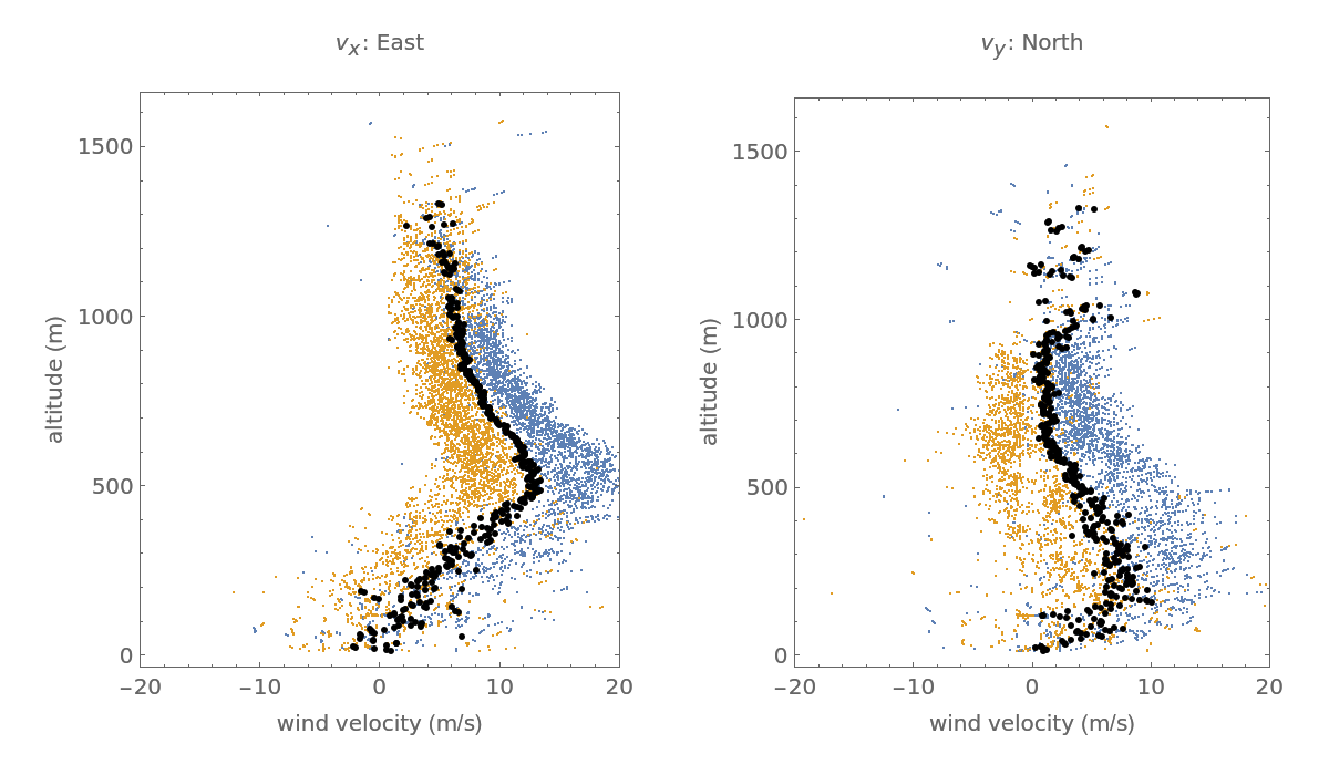
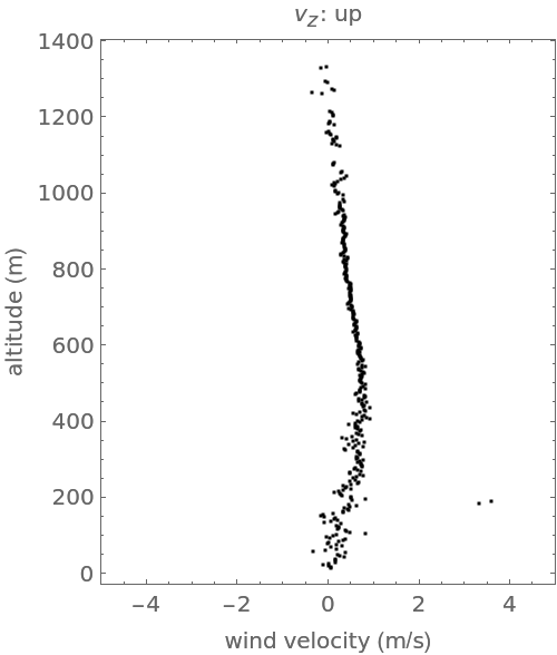
The least squares wind vector estimation algorithm is:The application of the algorithm to the data in the contact catalog lead to the following figure. The least squares solution is shown in black:The vertical component of the wind velocity vector is shown in the following:
![rd = ResourceData["Nocturnal Jet Wind Profiles Measured with WiPPR"];
a = ResourceData["Nocturnal Jet Wind Profiles Measured with WiPPR", "LogEchoMin"];
b = ResourceData["Nocturnal Jet Wind Profiles Measured with WiPPR", "LogEchoMax"];
VMin = ResourceData["Nocturnal Jet Wind Profiles Measured with WiPPR",
"VDopplerMin"];
VMax = ResourceData["Nocturnal Jet Wind Profiles Measured with WiPPR",
"VDopplerMax"];
dVDoppler = ResourceData["Nocturnal Jet Wind Profiles Measured with WiPPR", "dVDoppler"];
dz = ResourceData["Nocturnal Jet Wind Profiles Measured with WiPPR", "dz"];](https://www.wolframcloud.com/obj/resourcesystem/images/5b3/5b3a52ef-a337-4535-bb53-4fee4646c8d5/66fc56ed3311d43e.png)
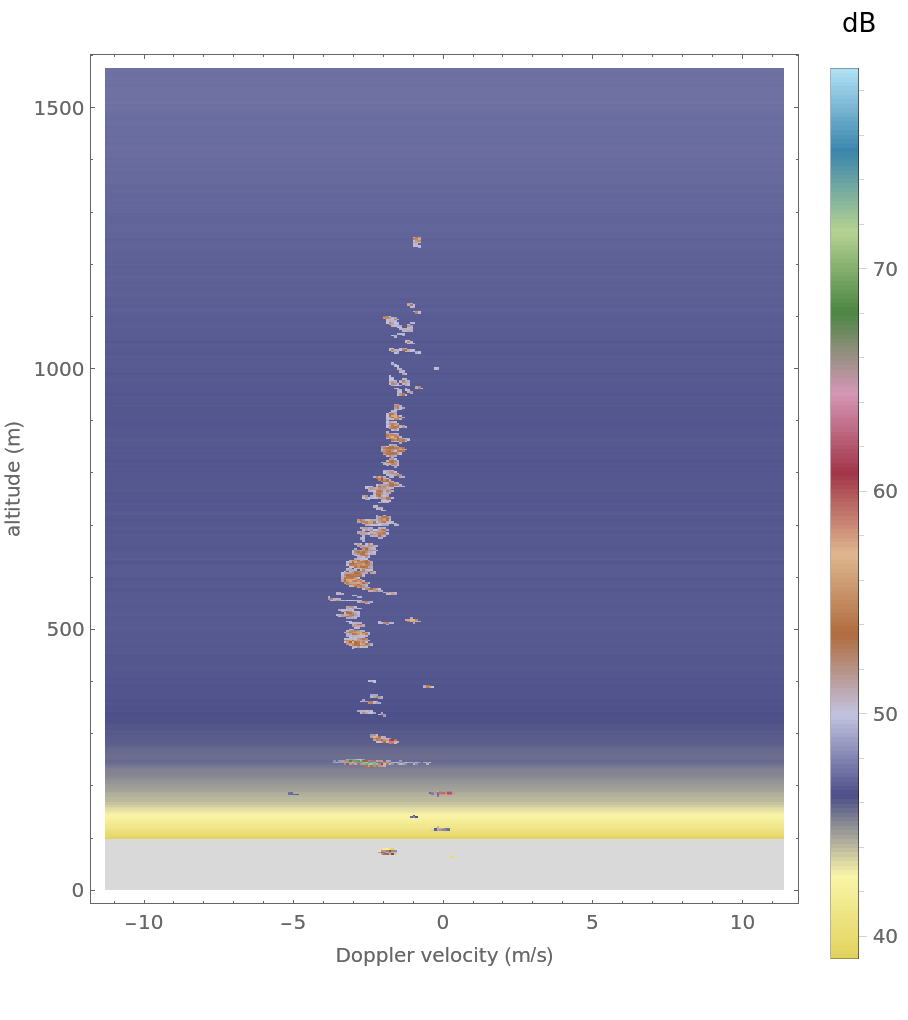
![nf = 30;
image = First@rd[[nf]];
rvm = Exp[ImageData[ImageReflect[ImageApply[(b*# + a) &, image]]]];
rvmdb = 10 Log[10, rvm]; dBplotmin = 39; dBplotmax = 79;
ReliefPlot[rvmdb, Sequence[
LightingAngle -> None, PlotRange -> {dBplotmin, dBplotmax}, ColorFunction -> ColorData[{"DarkBands", "Reverse"}], ClippingStyle -> {LightGray, Black}, FrameTicks -> Automatic, DataRange -> {{VMin, VMax}, {0, dz Length[rvmdb]}}, AspectRatio -> 1.2, FrameLabel -> {"Doppler velocity (m/s)", "altitude (m)"}, ImageSize -> 400, PlotLegends -> BarLegend[Automatic, LegendLabel -> "dB"]]]](https://www.wolframcloud.com/obj/resourcesystem/images/5b3/5b3a52ef-a337-4535-bb53-4fee4646c8d5/723149b23e143de6.png)
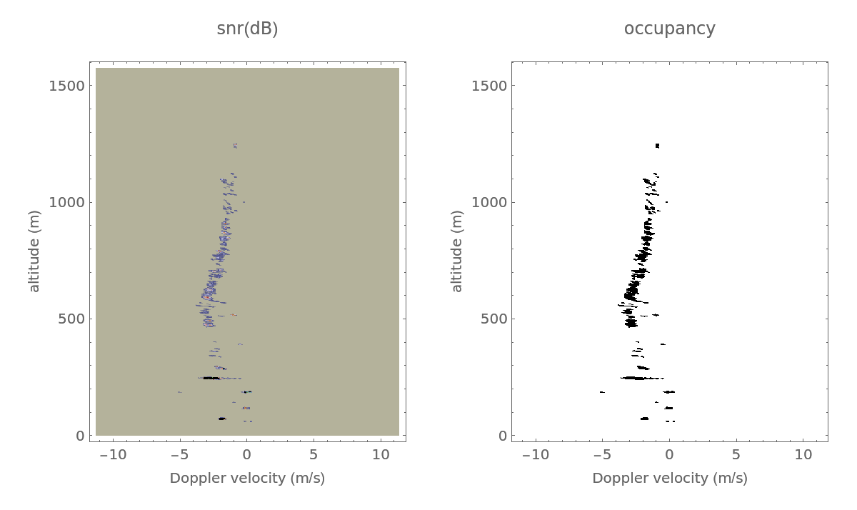
![snr = Map[#/Median[#] &, rvm];
SNRThresholdDB = 2;
occupancy = ImageData[Binarize[Image[snr], 10^(SNRThresholdDB/10)]];
snrdb = 10 Log[10, snr]; snrdbmax = Max[snrdb];
gsnr = ReliefPlot[snr, Sequence[
LightingAngle -> None, PlotRange -> {snrdbmax - 40, snrdbmax}, ColorFunction -> ColorData[{"DarkBands", "Reverse"}], ClippingStyle -> {Gray, Black}, FrameTicks -> Automatic, DataRange -> {{VMin, VMax}, {0, dz Length[rvmdb]}}, AspectRatio -> 1.2, FrameLabel -> {"Doppler velocity (m/s)", "altitude (m)"}, ImageSize -> 400, PlotLabel -> "snr(dB)"]];
gocc = ReliefPlot[occupancy, Sequence[
LightingAngle -> None, PlotRange -> {0.25, 0.5}, ClippingStyle -> {White, Black}, FrameTicks -> Automatic, DataRange -> {{VMin, VMax}, {0, dz Length[rvmdb]}}, AspectRatio -> 1.2, FrameLabel -> {"Doppler velocity (m/s)", "altitude (m)"}, ImageSize -> 400, PlotLabel -> "occupancy"]];
GraphicsRow[{gsnr, gocc}, ImageSize -> 600]](https://www.wolframcloud.com/obj/resourcesystem/images/5b3/5b3a52ef-a337-4535-bb53-4fee4646c8d5/0ae9933861e1201f.png)
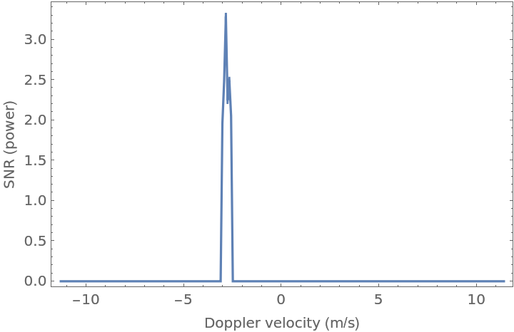
![nr = 152;
slice = snr[[nr]]*occupancy[[nr]];
If[Max[occupancy[[nr]]] > 0, pdf = slice/Total[slice]; Vecho = Table[ivv, {ivv, VMin, VMax, dVDoppler}]; Vest = pdf . Vecho;
position = Ceiling[(Vest - VMin)/dVDoppler]; If[position > 256, position = 256]; {Vest, nr*dz, snr[[nr, position]]}, "No echo greater than threshold"]](https://www.wolframcloud.com/obj/resourcesystem/images/5b3/5b3a52ef-a337-4535-bb53-4fee4646c8d5/551aa0f0b28428bc.png)
![WiPPRDataCatalog[rd_] := Module[{a, b, SNRThresholdDB = 2.0, dVDoppler, VDopplerlocal, image, thisbeam, \[Phi]Correct, \[Theta], \[Theta]Vertical, \[Eta], dzLcoal, cosX, cosY, cosZ, occupancy, rvm, snr, snrFiltered, goodRanges, zLocal, slice, pdf, Vpdf, catalog, catalogHeadings, VDopMin, VDopMax}, a = ResourceData["Nocturnal Jet Wind Profiles Measured with WiPPR", "LogEchoMin"]; b = ResourceData["Nocturnal Jet Wind Profiles Measured with WiPPR", "LogEchoMax"]; VDopMin = -11.3094; VDopMax = 11.3985; dVDoppler = (VDopMax - VDopMin)/255; VDopplerlocal = Table[V, {V, VDopMin, VDopMax, dVDoppler}]; catalog = Reap[Do[image = First@rd[[nf]]; thisbeam = Last@rd[[nf]]; \[Phi]Correct = (thisbeam - 1) \[Pi]/
2.0; \[Theta] = 80.0*\[Pi]/180.0; \[Theta]Vertical = \[Pi]/
2 - \[Theta]; \[Eta] = {Cos[\[Theta]] Sin[\[Phi]Correct], Cos[\[Theta]] Cos[\[Phi]Correct], Sin[\[Theta]]}; {cosX, cosY, cosZ} = Chop[\[Eta]]; dzLcoal = 3.125*Cos[\[Theta]Vertical]; rvm = Exp[
ImageData[ImageReflect[ImageApply[(b*# + a) &, image]]]]; snr = Map[#/Median[#] &, rvm]; occupancy = ImageData[Binarize[Image[snr], 10^(SNRThresholdDB/10)]]; snrFiltered = occupancy*snr; goodRanges = Map[First, Position[Map[Max, occupancy], 1]]; Do[zLocal = nRange*dzLcoal; slice = snrFiltered[[nRange]]; pdf = slice/Total[slice]; Vpdf = pdf . VDopplerlocal; Sow[Join[{zLocal, nf, Vpdf, cosX, cosY, cosZ, thisbeam}]], {nRange, goodRanges}], {nf, 1, Length[rd]}]]; catalog[[2]][[1]]]](https://www.wolframcloud.com/obj/resourcesystem/images/5b3/5b3a52ef-a337-4535-bb53-4fee4646c8d5/1311091983138d46.png)
![rd = ResourceData["Nocturnal Jet Wind Profiles Measured with WiPPR"];
catalog = WiPPRDataCatalog[rd];
catalogHeadings = {"z(m)", "nfile", "Vpdf(m/s)", "cosX", "cosY", "cosZ", "beam"};](https://www.wolframcloud.com/obj/resourcesystem/images/5b3/5b3a52ef-a337-4535-bb53-4fee4646c8d5/081faf7457cc1d32.png)

![ViewBeamDopplerData[catalog_, zmaxplot_] := Module[{cat, gD}, gD = Table[cat = Transpose@Select[catalog, #[[7]] == nbeam &]; ListPlot[Transpose[{cat[[3]], cat[[1]]}], Sequence[
PlotRange -> {{-11.3, 11.3}, {0, zmaxplot}}, Axes -> False, Frame -> True, AspectRatio -> 1., FrameLabel -> {"Doppler Velocity (m/s)", "Altitude (m)"}, PlotLabel -> Style[
ToString[nbeam], FontSize -> 9]], ImageSize -> 200], {nbeam, 1, 4}]; GraphicsGrid[{{gD[[1]], gD[[2]]}, {gD[[3]], gD[[4]]}}]]](https://www.wolframcloud.com/obj/resourcesystem/images/5b3/5b3a52ef-a337-4535-bb53-4fee4646c8d5/79f19494f9ebf934.png)
![ApparentVelocityBeamGrouped[catalog_] := Module[{\[Theta]Vertical, catT, catx4, catx2, caty1, caty3}, \[Theta]Vertical = ArcCos@First[catalog][[6]]; catT = Transpose@Select[catalog, #[[7]] == 4 &]; catx4 = Transpose[{catT[[3]]/Sin[\[Theta]Vertical], catT[[1]]}]; catT = Transpose@Select[catalog, #[[7]] == 2 &]; catx2 = Transpose[{-catT[[3]]/Sin[\[Theta]Vertical], catT[[1]]}]; catT = Transpose@Select[catalog, #[[7]] == 1 &]; caty1 = Transpose[{-catT[[3]]/Sin[\[Theta]Vertical], catT[[1]]}]; catT = Transpose@Select[catalog, #[[7]] == 3 &]; caty3 = Transpose[{catT[[3]]/Sin[\[Theta]Vertical], catT[[1]]}]; {{catx2, catx4}, {caty1, caty3}}]](https://www.wolframcloud.com/obj/resourcesystem/images/5b3/5b3a52ef-a337-4535-bb53-4fee4646c8d5/6113ee86fab069d7.png)
![{vxApparent, vyApparent} = ApparentVelocityBeamGrouped[catalog];
gx = ListPlot[vxApparent, Sequence[
PlotRange -> {{-20, 20}, All}, Axes -> False, Frame -> True, AspectRatio -> 1.2, FrameLabel -> {"wind velocity (m/s)", "altitude (m)"}, PlotLabel -> Style[
"\!\(\*SubscriptBox[\(v\), \(x\)]\): East", FontSize -> 10]]];
gy = ListPlot[vyApparent, Sequence[
PlotRange -> {{-20, 20}, All}, Axes -> False, Frame -> True, AspectRatio -> 1.2, FrameLabel -> {"wind velocity (m/s)", "altitude (m)"}, PlotLabel -> Style[
"\!\(\*SubscriptBox[\(v\), \(y\)]\): North", FontSize -> 10]]];
GraphicsRow[{gx, gy}, ImageSize -> 600]](https://www.wolframcloud.com/obj/resourcesystem/images/5b3/5b3a52ef-a337-4535-bb53-4fee4646c8d5/1efba9813d197ef6.png)
![LeastSquaresWindEstimates[catalog_, minUniqueBeams_ : 4] := Module[{zunique, tmp, cat, A, Aunique, Nbeams, V, vxL, vyL, vzL, z, vx, vy, vz}, zunique = Sort@DeleteDuplicates@Transpose[catalog][[1]]; tmp = Reap[
Do[cat = zunique[[nz]] /. GroupBy[catalog, First]; A = Map[Take[#, {4, 6}] &, cat]; Aunique = DeleteDuplicates@A; Nbeams = Length[Aunique]; If[Nbeams == minUniqueBeams, V = Transpose[cat][[3]]; {vxL, vyL, vzL} = -Inverse[Transpose[A] . A] . Transpose[A] . V; Sow[{zunique[[nz]], vxL, vyL, vzL}]], {nz, 1, Length[zunique]}]]; {z, vx, vy, vz} = Transpose@tmp[[2]][[1]]; {Transpose[{vx, z}], Transpose[{vy, z}], Transpose[{vz, z}]}]](https://www.wolframcloud.com/obj/resourcesystem/images/5b3/5b3a52ef-a337-4535-bb53-4fee4646c8d5/25bd2fa8e6532baa.png)
![{vxLS4, vyLS4, vzLS4} = LeastSquaresWindEstimates[catalog, 4];
gx = ListPlot[vxApparent, Sequence[
PlotRange -> {{-20, 20}, All}, Axes -> False, Frame -> True, AspectRatio -> 1.2, FrameLabel -> {"wind velocity (m/s)", "altitude (m)"}, PlotLabel -> Style[
"\!\(\*SubscriptBox[\(v\), \(x\)]\): East", FontSize -> 10]], Epilog -> {Point[vxLS4]}];
gy = ListPlot[vyApparent, Sequence[
PlotRange -> {{-20, 20}, All}, Axes -> False, Frame -> True, AspectRatio -> 1.2, FrameLabel -> {"wind velocity (m/s)", "altitude (m)"}, PlotLabel -> Style[
"\!\(\*SubscriptBox[\(v\), \(y\)]\): North", FontSize -> 10]], Epilog -> {Point[vyLS4]}];
GraphicsRow[{gx, gy}, ImageSize -> 600]](https://www.wolframcloud.com/obj/resourcesystem/images/5b3/5b3a52ef-a337-4535-bb53-4fee4646c8d5/49b1fc8dfb0a010c.png)