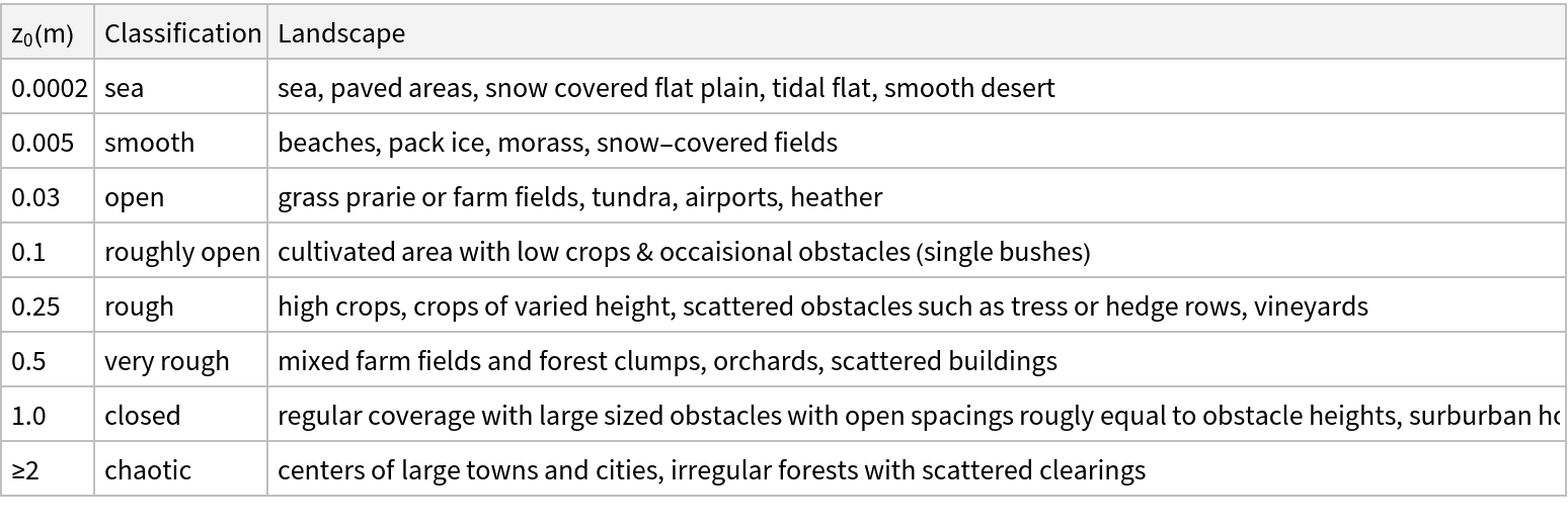
Parameters for Near Ground Wind Speed Estimation

Canopy height, surface roughness and Obukhov stability lengths for estimation of near-ground wind speed

Details

In a neutrally stable atmosphere the vertical wind profile u(z) at elevation z in the first 50-80 m above the ground has a logarithmic shape. Specifically κ u(z)/u_*=log(z/z₀) where κ=0.4 is the von Karman constant, u_* is the friction velocity and z₀ is the surface roughness. If τ is the surface stress exerted by the wind on the ground and ρ is air density then the friction velocity is u_*=(τ/ρ)^1/2. Application of the logarithmic profile requires z/z₀>>1.

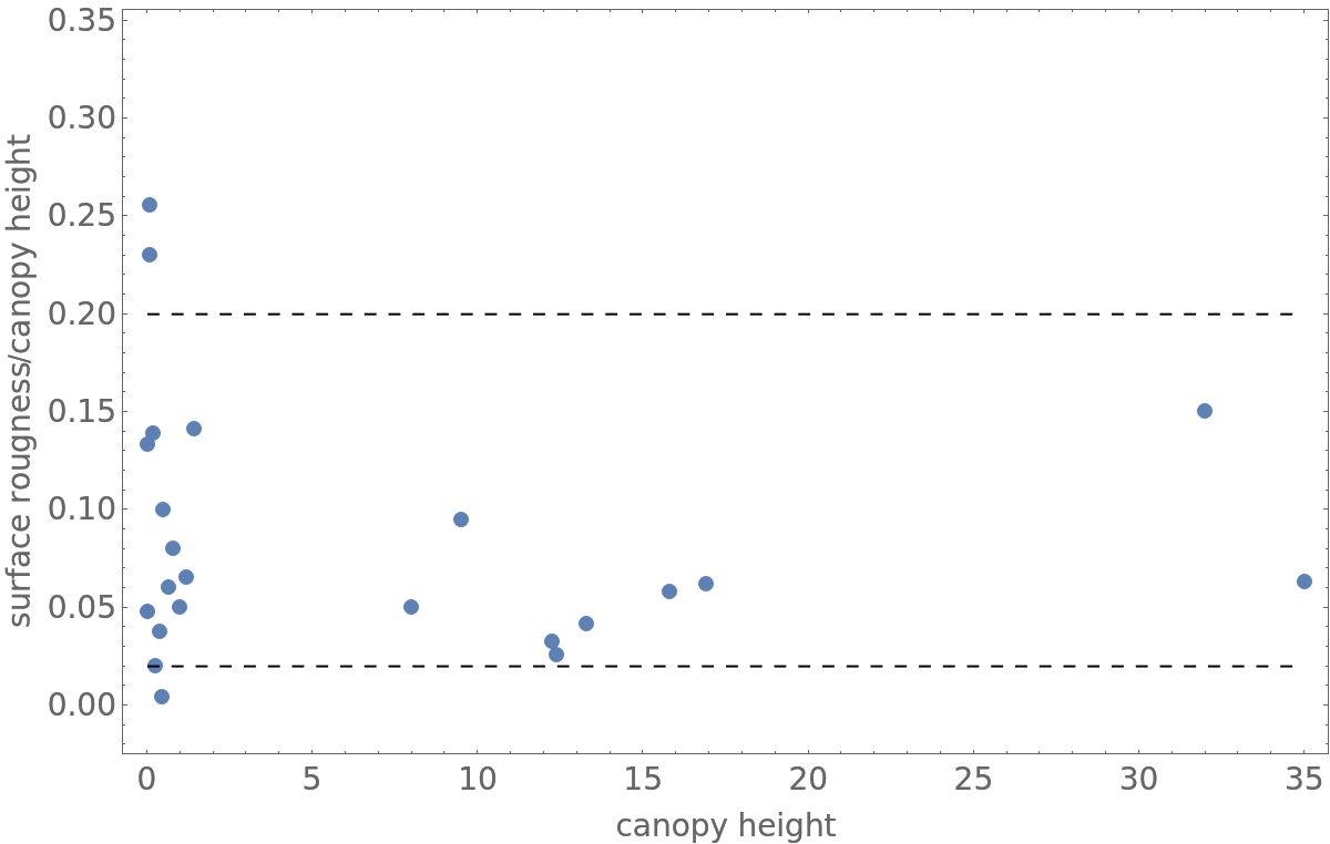
For surfaces with significant canopy height, e.g. tall tress, the form of the logarithmic profile must be modified for canopy effects. The modification is κ u(z)/u_*=log[(Z-d)/z₀] where Z is height above the substrate surface and d is the so-called zero plane displacement. For many naturally occurring surfaces the relationship between the canopy height h_c and the zero plane displacement d takes the simple form d/h_c≈2/3. The zero plane displacement values in the accompanying data table are expressed in the dimensionless form d/h_c.

For moderate wind speeds friction velocities are on the order of about 0.5 m/s. For strong winds friction velocities are on the order of 1.0 m/s. Friction velocity can be measured directly but it is usually inferred by making a wind speed measurement at a known height with an anemometer.

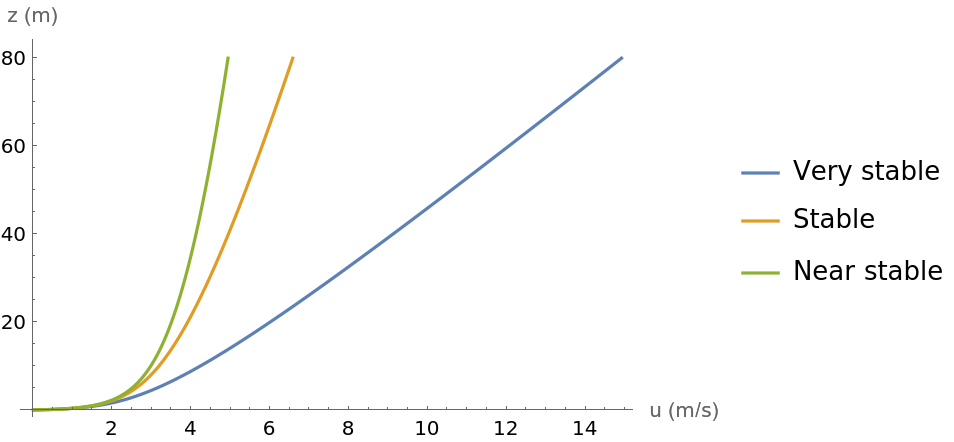
In a stable atmosphere wind speeds increase faster with altitude than predicted by the logarithmic profile. In an unstable environment the reverse happens. That is wind speeds increase slower with altitude than predicted by the logarithmic profile. The magnitude of these wind speed variations can be predicted using Monin-Obukhov similarity theory. This requires the introduction of an additional scale length, namely the Obukhov stability length L. In a stable atmosphere L>0 and the wind profile is approximately κ u(z)/u_*=log(z/z₀)+4.8z/L. In an unstable environment L<0 and an approximate form of the wind profile is κ u(z)/u_*=log(z/z₀)-3log(ψ(z)/ψ(z₀)) where ψ(z)=1+(1+3.6|z/L|)^1/2. If L becomes very large in a positive or negative sense then the Monin-Obukov profile reduces to the wind profile in a neutral atmosphere.

The Obukhov length L is defined via L=-u_*³/(κ (g/T_v)F) where u_* is the friction velocity, κ=0.4 is the von Karman constant, g is the acceleration due to gravity, T_v is the absolute virtual temperature and F is the kinematic surface heat flux. All the parameters in the equation defining the Obukhov length are positive with the exception of the kinematic surface heat flux F. Under stable conditions F<0 which makes L>0. Under unstable conditions F>0 and L<0. The Obukhov length can be interpreted as the height in a stable atmosphere where the production of turbulence by shear effects exceeds buoyant consumption. Stable conditions often occur at night. Unstable conditions often occur in daylight hours during time periods with high solar illumination.

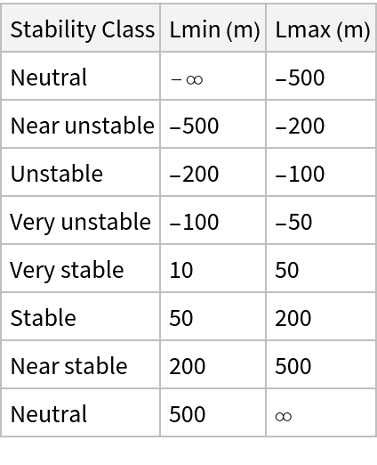
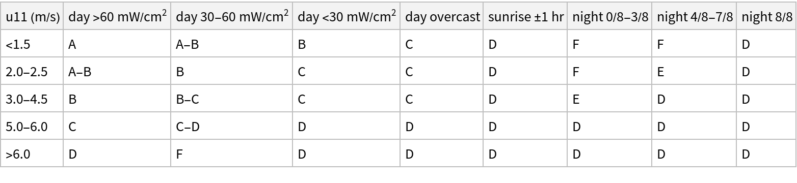
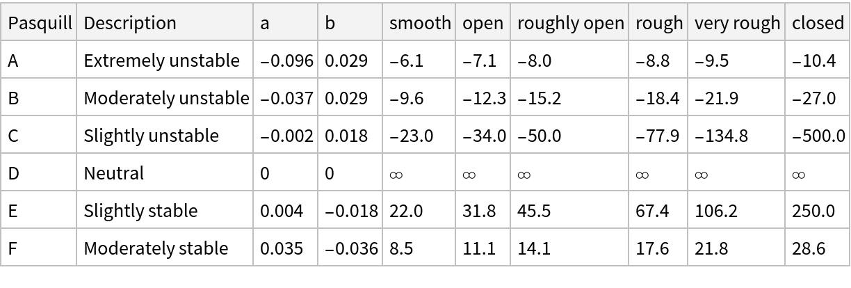
Atmospheric stability can be determined with the aid of the Pasquill meteorological stability estimation technique. The near-ground atmosphere is divided into 6 classes (A-F) and class determination is based upon observing the amount of incoming solar radiation in daylight (or cloud cover at night) and wind speed at a height of 11 m. Pasquill classes A, B and C occur in daylight hours and correspond to the most unstable and turbulent conditions. Class D typically corresponds to a neutral atmosphere which occurs near dawn. Classes E and F correspond to the most stable environments (typically at night) and least turbulent. Knowledge of the Pasquill stability class and surface roughness length z₀ can be used to estimate the Obukhov length L via the regression procedure L^-1=a+b log₁₀(z₀) where a and b are coefficients that depend on the Pasquill stability class.

(4 columns, 28 rows)

Examples

Basic Examples (2)

Display the basic data table that relates surface type to canopy height, roughness length and in a very few cases dimensionless zero plane displacement:

In[1]:=

$data = ResourceData[\!$\* TagBox["\"\<Parameters for Near Ground Wind Speed Estimation\>\"", #& , BoxID -> "ResourceTag-Parameters for Near Ground Wind Speed Estimation-Input", AutoDelete->True]$]$

Out[1]=

Parse through the data for the canopy height h_c and surface roughness z₀ and replace ranges in the data table with geometric means. Then plot the h_c versus z₀/h_c and verify that for most of the data the ratio lies on the range 0.02<z₀/h_c<0.2:

In[2]:=

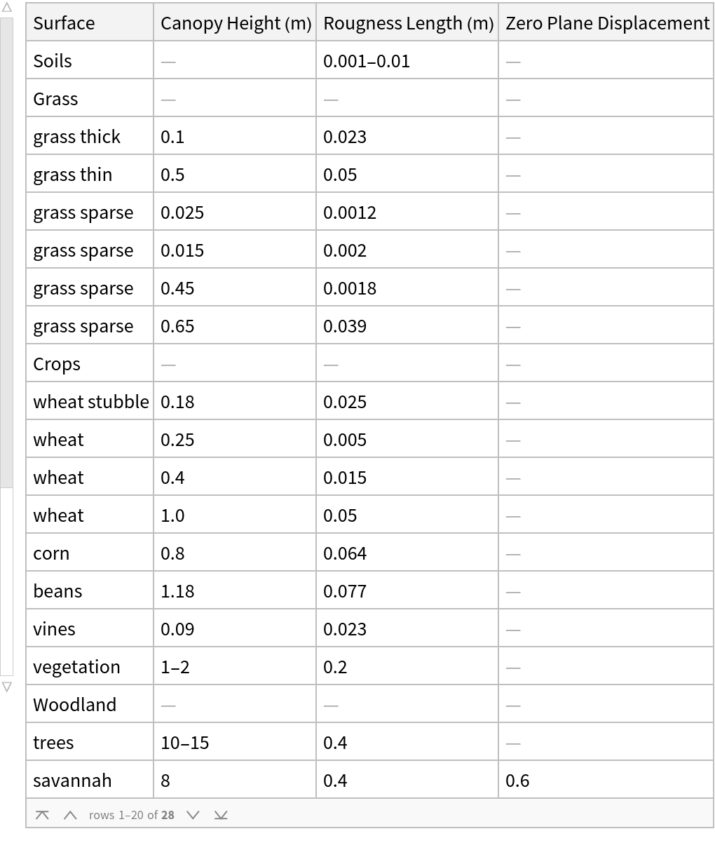
Clear[hc, all, missing, value, reformat, pairs];
hc = Normal@data[All, 2]; z0 = Normal@data[All, 3];
all = Transpose[{hc, z0}];
missing = Select[%, #[[1]] == Missing[] &];
value = Flatten[Complement[all, missing]];
reformat = If[NumberQ[#] == True, #, GeometricMean@ToExpression[StringSplit[#, "-"]] ] &;
pairs = Partition[Map[reformat, value], 2]; {hc, z0} = Transpose[pairs];
ListPlot[Transpose[{hc, z0/hc}], Sequence[
PlotRange -> {-0.025, Max[z0/hc] + 0.1}, Axes -> False, Frame -> True, FrameLabel -> {"canopy height", "surface rougness/canopy height"}, ImageSize -> 600, Epilog -> {{
Dashing[0.01],
Line[{{0, 0.02}, {35, 0.02}}]}, {
Dashing[0.01],
Line[{{0, 0.2}, {35, 0.2}}]}}, BaseStyle -> {FontSize -> 14}]]

Out[9]=

Scope & Additional Elements (4)

An approximate relationship between atmospheric stability and a range of Obukhov lengths (L_min,L_max) is described in the following table:

In[10]:=

$ResourceData[\!$\* TagBox["\"\<Parameters for Near Ground Wind Speed Estimation\>\"", #& , BoxID -> "ResourceTag-Parameters for Near Ground Wind Speed Estimation-Input", AutoDelete->True]$, "StabilityObukhovTable"]$

Out[10]=

The first step in making a wind speed profile estimate in the absence of measurements from a tall meteorological tower or balloon lifted radio sonde measurement is to estimate the atmospheric stability based upon observed local conditions at near-ground level. This requires observing the amount of incoming solar radiation in daylight (or amount of cloud cover in eighths at night) and estimating wind speed at a height of 11 m. With these values in hand the Pasquill stability class can be determined with the aid of the following table:

In[11]:=

Out[11]=

Next an estimate of surface roughness is required which characterizes the ground based upon the descriptors smooth, open, roughly open, rough, very rough and closed as used in the Davenport-Wieringa roughness is required:

In[12]:=

Out[12]=

Now it is possible to estimate the Obukhov length using the following table. The first column in the table is the Pasquill stability class. The second column relates the Pasquill class to stability descriptions. Columns 3 and 4 are the parameters in the expression L^-1=a+b log₁₀(z₀) where L is the Obukhov length and z₀ is the surface roughness in meters. Columns 5-10 are surface roughness descriptors from the Davenport-Wieringa table. The numerical entries in the table are Obukhov lengths in meters. Negative and positive values respectively correspond to unstable and stable atmospheric conditions:

In[13]:=

Out[13]=

Analysis (3)

Tabulate Obukhov stable lengths in stable environments using geometric means to replace data ranges:

In[14]:=

$data1 = ResourceData[\!$\* TagBox["\"\<Parameters for Near Ground Wind Speed Estimation\>\"", #& , BoxID -> "ResourceTag-Parameters for Near Ground Wind Speed Estimation-Input", AutoDelete->True]$, "StabilityObukhovTable"]; label = Take[Normal[data1[All, 1]], {5, 7}]; lmin = Take[Normal[data1[All, 2]], {5, 7}]; lmax = Take[Normal[data1[All, 3]], {5, 7}]; lObukhov = N@Map[GeometricMean, Transpose[{lmin, lmax}]]; Table[{label[[i]], lObukhov[[i]]}, {i, 1, 3}]; TableForm[%, TableHeadings -> {None, {"Stability", "(Lmin*Lmax\!$\*SuperscriptBox[\()$, $1/2$]\)"}}]$

Out[15]=

Plot wind speed profiles for the three cases in the foregoing example assuming a friction velocity of 0.25 m/s and a surface roughness of 0.1 m:

In[16]:=

$With[{ustar = 0.25, z0 = 0.1, \[Kappa] = 0.4}, profiles = Table[Table[{ustar/\[Kappa] (Log[z/z0] + 4.8 z/lObukhov[[i]]), z}, {z, z0, 80, 0.1}], {i, 1, 3}]]; ListLinePlot[profiles, Sequence[ PlotLegends -> label, AxesLabel -> {"u (m/s)", "z (m)"}]]$

Out[17]=

Compare wind profiles in a neutral, stable and unstable environment for a friction velocity of 0.5 m/s (very strong winds) and a surface roughness length of 0.1 m. Assume that the stability lengths for the very stable and very unstable environments are respectively 316 m and -71 m:

In[18]:=

$With[{ustar = 0.5, \[Kappa] = 0.4, z0 = 0.1, LStable = 316.0, \[Gamma]m = 3.6, LUnstable = -71}, profileNeutral = Table[{ustar/\[Kappa] Log[z/z0], z}, {z, z0, 80, 0.1}]; profileStable = Table[{ustar/\[Kappa] (Log[z/z0] + 4.8 z/LStable), z}, {z, z0, 80, 0.1}]; profileUntable = Table[{ustar/\[Kappa] (Log[z/z0] - 3 Log[(1 + (1 + \[Gamma]m*Abs[z/LUnstable])^(1/2))/( 1 + (1 + \[Gamma]m*Abs[z0/LUnstable])^(1/2))]), z}, {z, z0, 80, 0.1}]; ListLinePlot[{profileNeutral, profileStable, profileUntable}, Sequence[ PlotLegends -> {"Neutral", "Near stable", "Very unstable"}, AxesLabel -> {"u (m/s)", "z (m)"}]] ]$

Out[18]=

Bibliographic Citation

Marshall Bradley, "Parameters for Near Ground Wind Speed Estimation" from the Wolfram Data Repository (2022)

Data Resource History

Date Created: 28 October 2022

Source Metadata

Citation:
- Garratt, J. R. (1992), The Atmospheric Boundary Layer, Cambridge University Press.

Publisher Information

Prepared for the Wolfram Data Repository By: Marshall Bradley
Publisher of Record: Marshall Bradley