Wolfram Data Repository
Immediate Computable Access to Curated Contributed Data
Half lives in seconds for 1175 radioactive isotopes
Retrieve the data and present the the data in a tabular format:
| In[1]:= |
| Out[1]= | 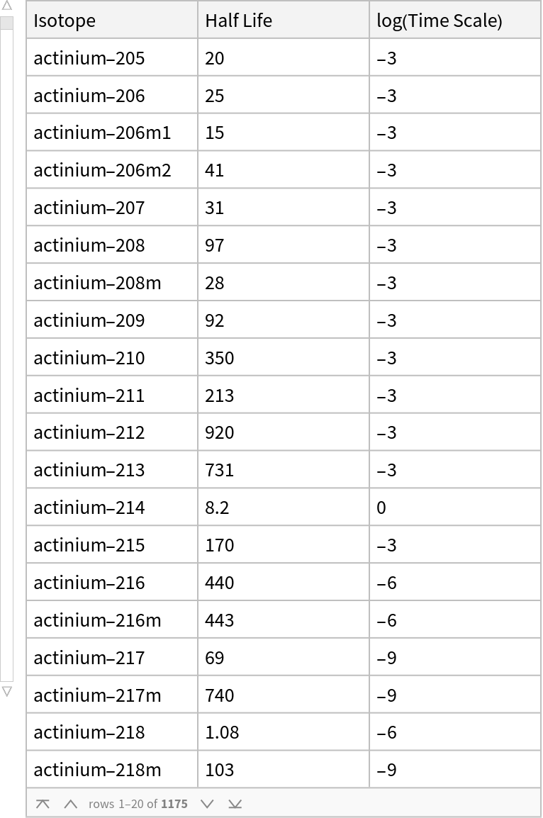 |
Display all entries in the data set for the element bismuth with half lives in seconds converted to a log scale:
| In[2]:= | ![element = "bismuth";
dataset = ResourceData[\!\(\*
TagBox["\"\<Radioactive Isotope Half Lives\>\"",
#& ,
BoxID -> "ResourceTag-Radioactive Isotope Half Lives-Input",
AutoDelete->True]\)];
name = dataset[All, "Isotope"] // Normal;
x = dataset[All, "Half Life"] // Normal; y = dataset[All, "log(Time Scale)"] // Normal;
{elmnt, iso} = Transpose[Map[StringSplit[#, "-"] &, name]];
data = Transpose[{elmnt, iso, Log[10, N[x*10^y]]}]; data = Select[data, #[[1]] == element &];
temp = Table[<|"Element" -> data[[i]][[1]], "Isotope Number" -> data[[i]][[2]], "Log[10,Half Life (sec)]" -> data[[i]][[3]]|>, {i, 1, Length[data]}];
Dataset[temp, ItemSize -> 18]](https://www.wolframcloud.com/obj/resourcesystem/images/eec/eec66a63-6de1-4dfe-839a-afeed6e3a377/519302d69a2ab724.png) |
| Out[9]= |  |
The following block of code compares the observed distribution of first digits in the half life data set to the theoretical Bedford distribution. The agreement is quite good:
| In[10]:= | ![dataset = ResourceData[\!\(\*
TagBox["\"\<Radioactive Isotope Half Lives\>\"",
#& ,
BoxID -> "ResourceTag-Radioactive Isotope Half Lives-Input",
AutoDelete->True]\)];
firstdigits = dataset[All, "Half Life"] // Normal;
firstdigit = Map[ToExpression, Map[First, Map[Characters, Map[ToString, firstdigits]]]];
counts = Table[Count[firstdigit, i], {i, 1, 9}];
measured = N@counts/Total[counts];
theoretical = Map[Point, N@Table[{i, Log[10, (i + 1)/i]}, {i, 1, 9}]];
ref = Line[Table[{i, Log[10, (i + 1)/i]}, {i, 1, 9, 0.01}]];
BarChart[measured, Epilog -> {PointSize[0.025], theoretical, ref}, PlotRange -> {0, 0.350}, ChartLabels -> Placed[{1, 2, 3, 4, 5, 6, 7, 8, 9}, Bottom]]](https://www.wolframcloud.com/obj/resourcesystem/images/eec/eec66a63-6de1-4dfe-839a-afeed6e3a377/674634d08954b2d0.png) |
| Out[17]= | 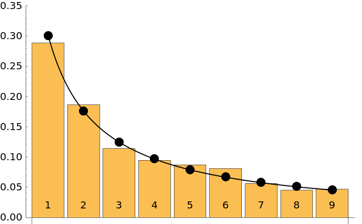 |
Marshall Bradley, "Radioactive Isotope Half Lives" from the Wolfram Data Repository (2024)