Wolfram Data Repository
Immediate Computable Access to Curated Contributed Data
Locations of the 1854 London cholera outbreak near Golden Square
| In[1]:= |
| Out[1]= | 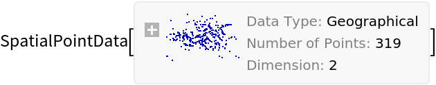 |
Summary of the spatial point data:
| In[2]:= |
| Out[2]= | 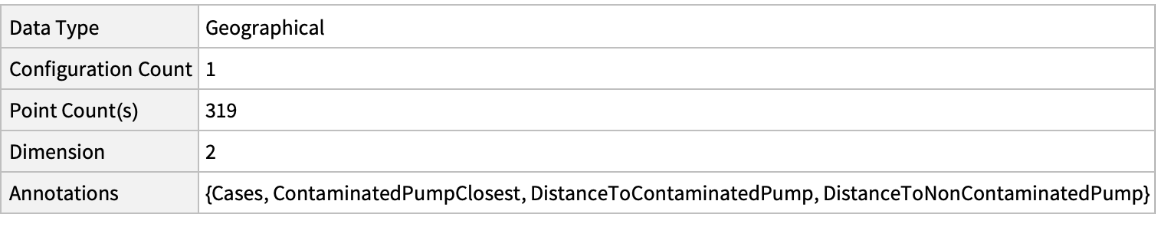 |
Plot the locations:
| In[3]:= |
| Out[3]= | 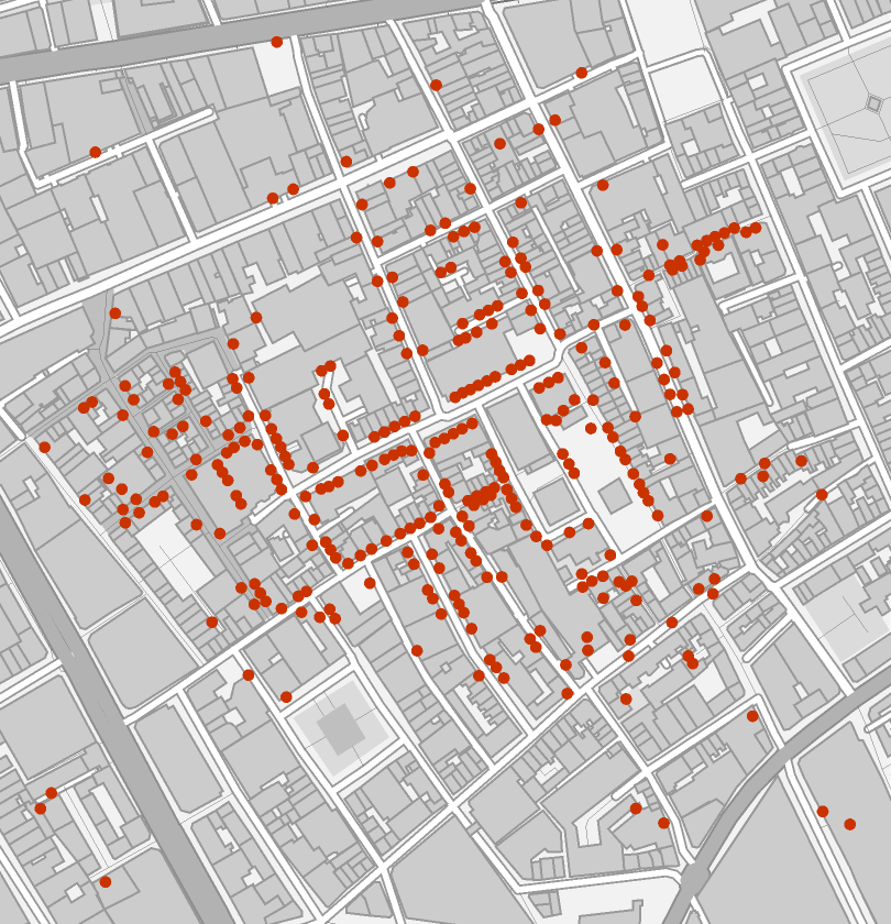 |
Visualize the number of cases per location with information whether the contaminated pump was the closest:
| In[4]:= | ![legend = With[{cases = Union[ResourceData[\!\(\*
TagBox["\"\<Sample Data: London Cholera\>\"",
#& ,
BoxID -> "ResourceTag-Sample Data: London Cholera-Input",
AutoDelete->True]\), "Data"][{"Annotations", "Cases"}][[1]]]}, PointLegend[ColorData[97, "ColorList"][[1 ;; Length[cases]]], cases, LegendLabel -> "number of cases \n per location", LegendMarkerSize -> 20, LegendFunction -> Frame]];](https://www.wolframcloud.com/obj/resourcesystem/images/ff1/ff1057f3-620f-41e6-8dd2-176a09049c59/5e2609ba4d70e58f.png) |
| In[5]:= | ![Legended[PointValuePlot[ResourceData[\!\(\*
TagBox["\"\<Sample Data: London Cholera\>\"",
#& ,
BoxID -> "ResourceTag-Sample Data: London Cholera-Input",
AutoDelete->True]\), "Data"], {1 -> Automatic, 2 -> None, 3 -> None, 4 -> None}, GeoBackground -> "VectorMonochrome"], legend]](https://www.wolframcloud.com/obj/resourcesystem/images/ff1/ff1057f3-620f-41e6-8dd2-176a09049c59/42e9655b2bedc90a.png) |
| Out[5]= | 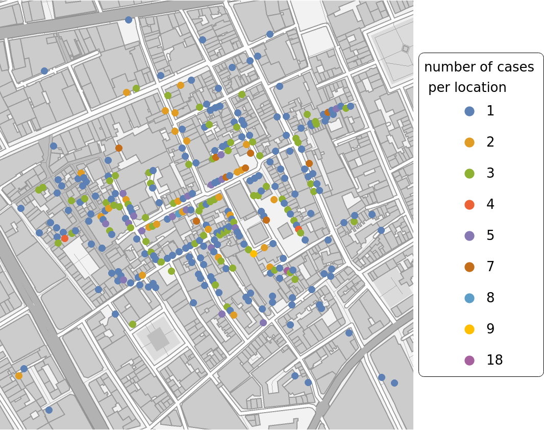 |
Compute probability of finding a point within given radius of an existing point - NearestNeighborG is the CDF of the nearest neighbor distribution:
| In[6]:= |
| Out[6]= | 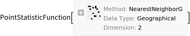 |
| In[7]:= |
| Out[7]= |
| In[8]:= |
| Out[8]= |
| In[9]:= |
| Out[9]= | 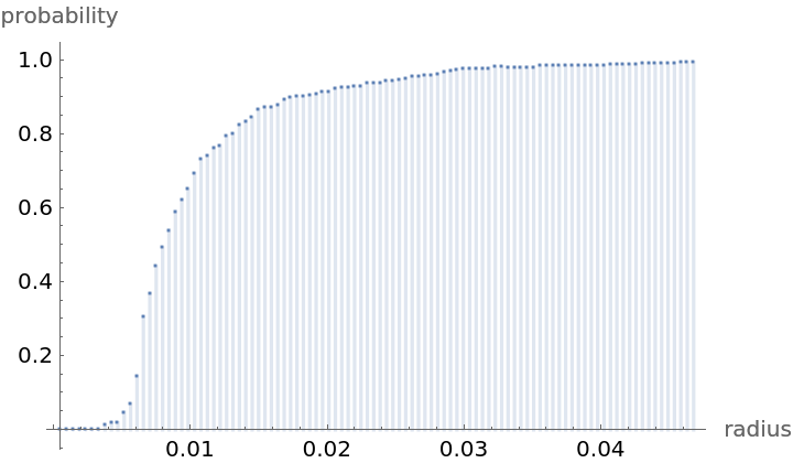 |
NearestNeighborG as the CDF of nearest neighbor distribution can be used to compute the mean distance between a typical point and its nearest neighbor - the mean of a positive support distribution can be approximated via a Riemann sum of 1- CDF. To use Riemann approximation create the partition of the support interval from 0 to maxR into 100 parts and compute the value of the NearestNeighborG at the middle of each subinterval:
| In[10]:= | ![step = maxR/100;
middles = Subdivide[step/2, maxR - step/2, 99];
values = nnG[middles];](https://www.wolframcloud.com/obj/resourcesystem/images/ff1/ff1057f3-620f-41e6-8dd2-176a09049c59/6d1b218e41414834.png) |
Now compute the Riemann sum to find the mean distance between a typical point and its nearest neighbor:
| In[11]:= |
| Out[11]= |
Test for complete spacial randomness:
| In[12]:= |
| Out[12]= |
Gosia Konwerska, "Sample Data: London Cholera" from the Wolfram Data Repository (2022)