Examples
Basic Examples (1)
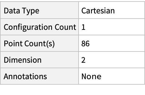
Summary of the spatial point data:
Visualizations (2)
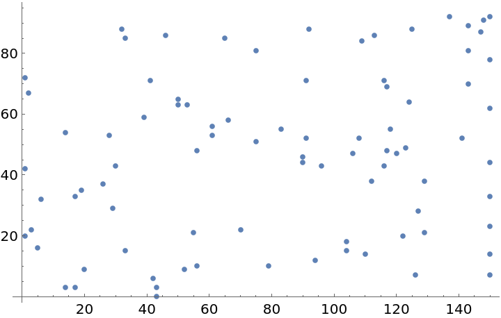
Plot the spatial point data:
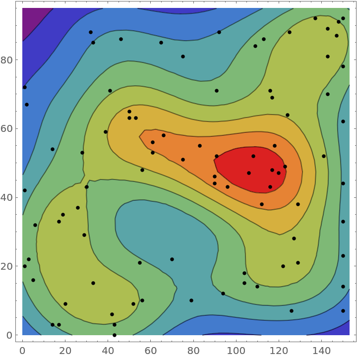
Visualize smooth point density of the data:
Analysis (6)
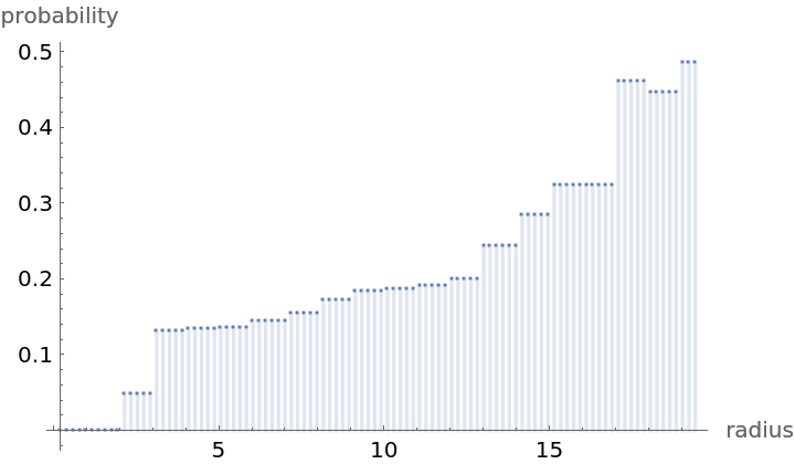
Compute probability of finding a point within given radius of an existing point - NearestNeighborG is the CDF of the nearest neighbor distribution:
NearestNeighborG as the CDF of nearest neighbor distribution can be used to compute the mean distance between a typical point and its nearest neighbor - the mean of a positive support distribution can be approximated via a Riemann sum of 1- CDF. To use Riemann approximation create the partition of the support interval from 0 to maxR into 100 parts and compute the value of the NearestNeighborG at the middle of each subinterval:
Now compute the Riemann sum to find the mean distance between a typical point and its nearest neighbor:
Account for scale and units:
Test for complete spacial randomness:
Fit a Poisson point process to the data:
Bibliographic Citation
Gosia Konwerska,
"Sample Data: NZ Trees"
from the Wolfram Data Repository
(2022)
Data Resource History
Publisher Information


![Show[ContourPlot[density[{x, y}], {x, y} \[Element] ResourceData[\!\(\*
TagBox["\"\<Sample Data: NZ Trees\>\"",
#& ,
BoxID -> "ResourceTag-Sample Data: NZ Trees-Input",
AutoDelete->True]\), "ObservationRegion"], ColorFunction -> "Rainbow"], ListPlot[ResourceData[\!\(\*
TagBox["\"\<Sample Data: NZ Trees\>\"",
#& ,
BoxID -> "ResourceTag-Sample Data: NZ Trees-Input",
AutoDelete->True]\), "Data"], PlotStyle -> Black]]](https://www.wolframcloud.com/obj/resourcesystem/images/91e/91edd5b0-d163-4c9c-8589-9d945512ff08/6d16d314c591dbca.png)

![step = maxR/100;
middles = Subdivide[step/2, maxR - step/2, 99];
values = nnG[middles];](https://www.wolframcloud.com/obj/resourcesystem/images/91e/91edd5b0-d163-4c9c-8589-9d945512ff08/74bcb152e5bd030f.png)