Wolfram Data Repository
Immediate Computable Access to Curated Contributed Data
Locations of murders in Toronto annotated with marks including victim age, victim sex, type, murder method, and year
| In[1]:= |
| Out[1]= | 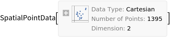 |
Summary of the spatial point data:
| In[2]:= |
| Out[2]= | 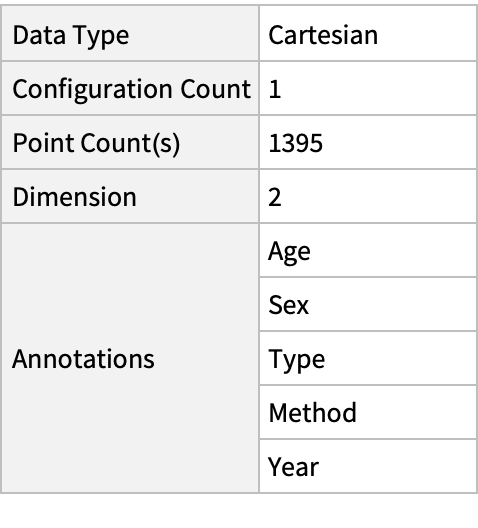 |
Plot the spatial point data:
| In[3]:= |
| Out[3]= | 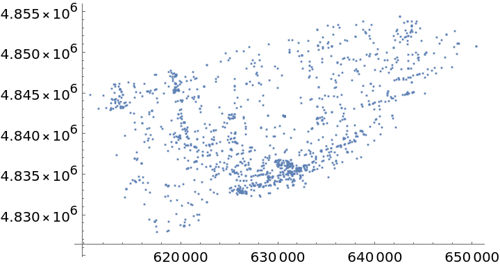 |
Visualize the smooth point density:
| In[4]:= |
| Out[4]= | 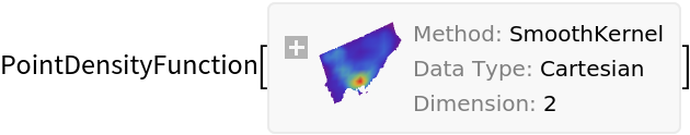 |
| In[5]:= | ![Show[density["DensityVisualization"], ListPlot[ResourceData[\!\(\*
TagBox["\"\<Sample Data: Toronto Murders\>\"",
#& ,
BoxID -> "ResourceTag-Sample Data: Toronto Murders-Input",
AutoDelete->True]\), "Data"], PlotStyle -> Black], Frame -> True]](https://www.wolframcloud.com/obj/resourcesystem/images/8ab/8abda1c4-e744-4561-b88a-7730d60829e6/364797a0dbc76f63.png) |
| Out[5]= | 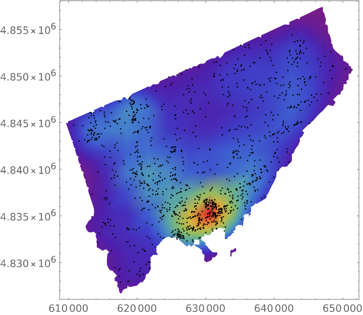 |
Visualize the data with annotations:
| In[6]:= | ![Show[Graphics[{Opacity[.2], ResourceData[\!\(\*
TagBox["\"\<Sample Data: Toronto Murders\>\"",
#& ,
BoxID -> "ResourceTag-Sample Data: Toronto Murders-Input",
AutoDelete->True]\), "ObservationRegion"]}], PointValuePlot[ResourceData[\!\(\*
TagBox["\"\<Sample Data: Toronto Murders\>\"",
#& ,
BoxID -> "ResourceTag-Sample Data: Toronto Murders-Input",
AutoDelete->True]\), "Data"], {1 -> None, 2 -> Automatic, 3 -> None, 4 -> None, 5 -> None}, PlotLegends -> Automatic], PlotLabel -> "Victim sex"]](https://www.wolframcloud.com/obj/resourcesystem/images/8ab/8abda1c4-e744-4561-b88a-7730d60829e6/6ba2ec7fa5526f82.png) |
| Out[6]= | 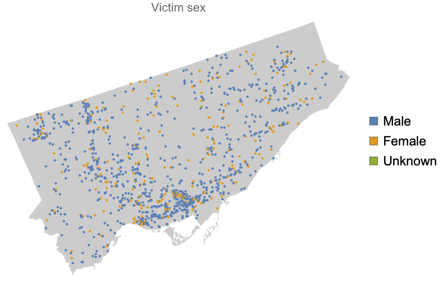 |
Compute probability of finding a point within given radius of an existing point - NearestNeighborG is the CDF of the nearest neighbor distribution:
| In[7]:= |
| Out[7]= | 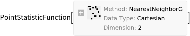 |
| In[8]:= |
| Out[8]= |
| In[9]:= |
| Out[9]= | 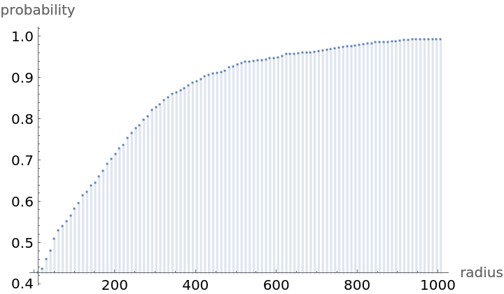 |
NearestNeighborG as the CDF of nearest neighbor distribution can be used to compute the mean distance between a typical point and its nearest neighbor - the mean of a positive support distribution can be approximated via a Riemann sum of 1- CDF. To use Riemann approximation create the partition of the support interval from 0 to maxR into 100 parts and compute the value of the NearestNeighborG at the middle of each subinterval:
| In[10]:= | ![step = maxR/100;
middles = Subdivide[step/2, maxR - step/2, 99];
values = nnG[middles];](https://www.wolframcloud.com/obj/resourcesystem/images/8ab/8abda1c4-e744-4561-b88a-7730d60829e6/691ccaa167d54b71.png) |
Now compute the Riemann sum to find the mean distance between a typical point and its nearest neighbor:
| In[11]:= |
| Out[11]= |
Test for complete spatial randomness:
| In[12]:= |
| Out[12]= |  |
Fit a Poisson point process to data:
| In[13]:= | ![Clear[\[Mu]];
EstimatedPointProcess[ResourceData[\!\(\*
TagBox["\"\<Sample Data: Toronto Murders\>\"",
#& ,
BoxID -> "ResourceTag-Sample Data: Toronto Murders-Input",
AutoDelete->True]\), "Data"], PoissonPointProcess[\[Mu], 2]]](https://www.wolframcloud.com/obj/resourcesystem/images/8ab/8abda1c4-e744-4561-b88a-7730d60829e6/59fc27cfe13dd6c0.png) |
| Out[14]= |
Gosia Konwerska, "Sample Data: Toronto Murders" from the Wolfram Data Repository (2022)