Wolfram Data Repository
Immediate Computable Access to Curated Contributed Data
Total ozone over the US measured on 5 August 2021
| In[1]:= |
| Out[1]= |  |
Summary of the spatial point data:
| In[2]:= |
| Out[2]= | 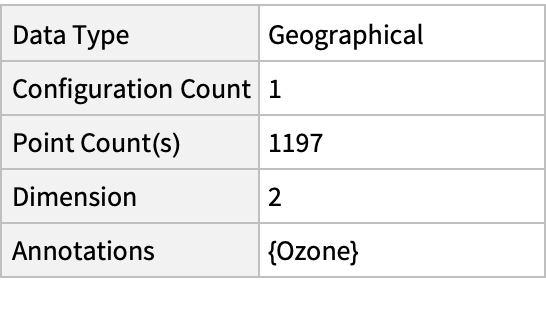 |
Plot the spatial point data:
| In[3]:= | ![Legended[PointValuePlot[ResourceData[\!\(\*
TagBox["\"\<Sample Data: US Ozone 2021\>\"",
#& ,
BoxID -> "ResourceTag-Sample Data: US Ozone 2021-Input",
AutoDelete->True]\), "Data"], ColorFunction -> "Rainbow"], BarLegend[{"Rainbow", MinMax[ResourceData[\!\(\*
TagBox["\"\<Sample Data: US Ozone 2021\>\"",
#& ,
BoxID -> "ResourceTag-Sample Data: US Ozone 2021-Input",
AutoDelete->True]\), "Annotations"]]}]]](https://www.wolframcloud.com/obj/resourcesystem/images/b40/b40d4a13-3cdf-4cf6-aeb2-c6af33bb3e9a/72a055856471771c.png) |
| Out[3]= | 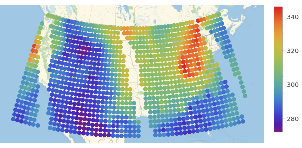 |
Use SpatialEstimate to create a continuous estimate from sparse observation locations:
| In[4]:= |
| Out[4]= |  |
| In[5]:= | ![pts = RandomGeoPosition[ResourceData[\!\(\*
TagBox["\"\<Sample Data: US Ozone 2021\>\"",
#& ,
BoxID -> "ResourceTag-Sample Data: US Ozone 2021-Input",
AutoDelete->True]\), "Data"]["ObservationRegion"], 2000];
vals = est[pts];](https://www.wolframcloud.com/obj/resourcesystem/images/b40/b40d4a13-3cdf-4cf6-aeb2-c6af33bb3e9a/5291c95875320f4d.png) |
Visualize rainfall values over the whole region:
| In[6]:= |
| Out[6]= | 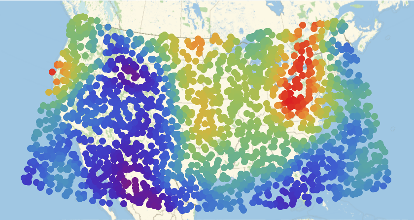 |
Gosia Konwerska, "Sample Data: US Ozone 2021" from the Wolfram Data Repository (2022)