Wolfram Data Repository
Immediate Computable Access to Curated Contributed Data
Images of turbulent wind motions moving through a near vertical beam of an FMCW radar recorded near Palm Canyon Arizona
| "CarrierFrequency" | radar carrier frequency (GHz) |
| "CandWidth" | radar bandwidth (MHz) |
| "PulseLength" | radar pulse length (sec) |
| "θVertical" | radar angle with respect to the vertical (deg) |
| "MaxDopplerVelocity" | maximum Doppler velocity (m/s) |
| "MaxAltitude" | max altitude sampled by radar (m) |
| "MaxSlowTime" | time span of radar images (sec) |
Retrieve the data at a particular altitude:
| In[1]:= | ![nz = 100;
images = ResourceData[\!\(\*
TagBox["\"\<WiPPR Images of Convective Boundary Layer Turbulence\>\"",
#& ,
BoxID -> "ResourceTag-WiPPR Images of Convective Boundary Layer Turbulence-Input",
AutoDelete->True]\)];
image = images[[nz]]](https://www.wolframcloud.com/obj/resourcesystem/images/ab7/ab7741c7-1eaa-4e97-8321-c35716d14e40/72491c3bce61b952.png) |
| Out[3]= | 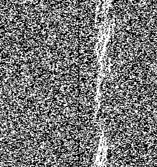 |
Display top 30 db range of data at an altitude with slow time (recording time) increasing from bottom of image to the top:
| In[4]:= | ![datadb = ImageData[image];
{mindb, maxdb} = MinMax[datadb];
vmax = ResourceData[\!\(\*
TagBox["\"\<WiPPR Images of Convective Boundary Layer Turbulence\>\"",
#& ,
BoxID -> "ResourceTag-WiPPR Images of Convective Boundary Layer Turbulence-Input",
AutoDelete->True]\), "MaxDopplerVelocity"];
tmax = ResourceData[\!\(\*
TagBox["\"\<WiPPR Images of Convective Boundary Layer Turbulence\>\"",
#& ,
BoxID -> "ResourceTag-WiPPR Images of Convective Boundary Layer Turbulence-Input",
AutoDelete->True]\), "MaxSlowTime"];
ReliefPlot[datadb, PlotRange -> {maxdb - 30, maxdb}, Sequence[
LightingAngle -> None, FrameTicks -> True, DataRange -> {{-vmax, vmax}, {0, tmax}}, FrameLabel -> {"Doppler velocity (m/s)", "slow time (sec)"}]]](https://www.wolframcloud.com/obj/resourcesystem/images/ab7/ab7741c7-1eaa-4e97-8321-c35716d14e40/2e53997fec72c561.png) |
| Out[5]= | 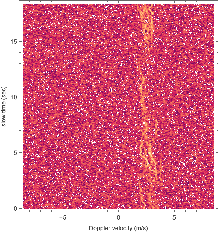 |
Set an SNR threshold and use morphological processing to clean the image up:
| In[6]:= | ![SNRThresholdDB = 7.0;
SmallComponentSize = 10;
binaryImage = Binarize[Image[datadb], SNRThresholdDB];
mask = DeleteSmallComponents[binaryImage, SmallComponentSize];
datadbClean = ImageData[mask] datadb;
ReliefPlot[datadbClean, PlotRange -> {maxdb - 30, maxdb}, Sequence[
LightingAngle -> None, FrameTicks -> True, DataRange -> {{-vmax, vmax}, {0, tmax}}, FrameLabel -> {"Doppler velocity (m/s)", "slow time (sec)"}]]](https://www.wolframcloud.com/obj/resourcesystem/images/ab7/ab7741c7-1eaa-4e97-8321-c35716d14e40/6c37d5da1e50f1cf.png) |
| Out[7]= | 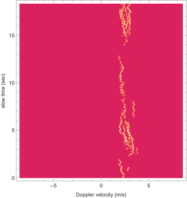 |
Marginalize (sum binary images) across altitude to summarize the temporal structure of the turbulence:
| In[8]:= | ![imagenames = ResourceData[\!\(\*
TagBox["\"\<WiPPR Images of Convective Boundary Layer Turbulence\>\"",
#& ,
BoxID -> "ResourceTag-WiPPR Images of Convective Boundary Layer Turbulence-Input",
AutoDelete->True]\)];
vmax = ResourceData[\!\(\*
TagBox["\"\<WiPPR Images of Convective Boundary Layer Turbulence\>\"",
#& ,
BoxID -> "ResourceTag-WiPPR Images of Convective Boundary Layer Turbulence-Input",
AutoDelete->True]\), "MaxDopplerVelocity"];
tmax = ResourceData[\!\(\*
TagBox["\"\<WiPPR Images of Convective Boundary Layer Turbulence\>\"",
#& ,
BoxID -> "ResourceTag-WiPPR Images of Convective Boundary Layer Turbulence-Input",
AutoDelete->True]\), "MaxSlowTime"];
SNRThresholdDB = 10.0;
SmallComponentSize = 10;
altitudeMarginalization = Sum[
datadb = ImageData[imagenames[[nz]]];
binaryImage = Binarize[Image[datadb], SNRThresholdDB];
mask = DeleteSmallComponents[binaryImage, SmallComponentSize];
ImageData[mask], {nz, 4, 124, 4}];
ReliefPlot[altitudeMarginalization, Sequence[PlotRange -> {1,
Max[altitudeMarginalization]}, LightingAngle -> None, FrameLabel -> {"Doppler velocity (m/s)", "slow time (sec)"}, BaseStyle -> {FontFamily -> "Arial", FontSize -> 12}, DataRange -> {{-vmax, vmax}, {0, tmax}}, FrameTicks -> True, ImageSize -> 400, AspectRatio -> 1, ClippingStyle -> {Black, Red}, PlotLegends -> BarLegend[
Automatic, LegendLabel -> Style["count", FontSize -> 10]]]]](https://www.wolframcloud.com/obj/resourcesystem/images/ab7/ab7741c7-1eaa-4e97-8321-c35716d14e40/2b7cee2df5b347c0.png) |
| Out[9]= | 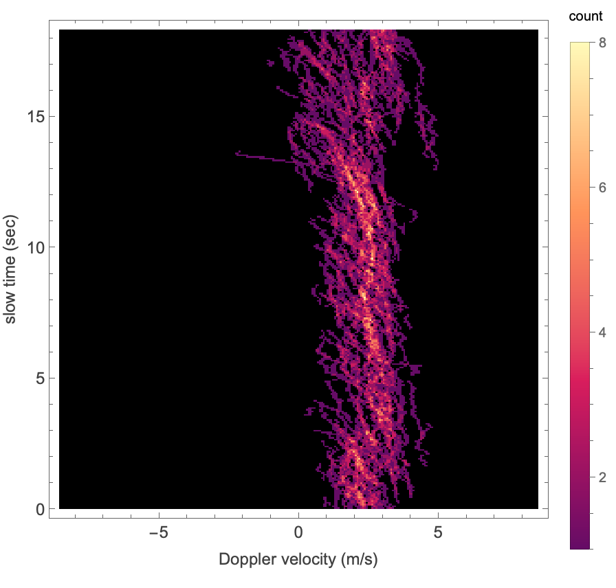 |
Marginalize across slow time to reveal the wind profile:
| In[10]:= | ![SNRThresholdDB = 10.0;
SmallComponentSize = 10;
zmax = ResourceData[\!\(\*
TagBox["\"\<WiPPR Images of Convective Boundary Layer Turbulence\>\"",
#& ,
BoxID -> "ResourceTag-WiPPR Images of Convective Boundary Layer Turbulence-Input",
AutoDelete->True]\), "MaxAltitude"];
datacube = Table[
datadb = ImageData[imagenames[[nz]]];
binaryImage = Binarize[Image[datadb], SNRThresholdDB];
mask = DeleteSmallComponents[binaryImage, SmallComponentSize];
ImageData[mask], {nz, 1, 129, 3}];
datacube = Transpose[datacube];
slowtimeMarginalization = Sum[datacube[[nt]], {nt, 1, Length[datacube]}];
ReliefPlot[slowtimeMarginalization, Sequence[PlotRange -> {1,
Max[slowtimeMarginalization]}, LightingAngle -> None, BaseStyle -> {FontFamily -> "Arial", FontSize -> 12}, AspectRatio -> 1, FrameTicks -> True, ImageSize -> 400, ClippingStyle -> {Black, Black}, DataRange -> {{-vmax, vmax}, {0, zmax}}, FrameLabel -> {"Doppler velocity (m/s)", "altitude (m)"}, PlotLegends -> BarLegend[
Automatic, LegendLabel -> Style["Count", FontSize -> 10]]]]](https://www.wolframcloud.com/obj/resourcesystem/images/ab7/ab7741c7-1eaa-4e97-8321-c35716d14e40/5b051c7f93eefb7d.png) |
| Out[11]= | 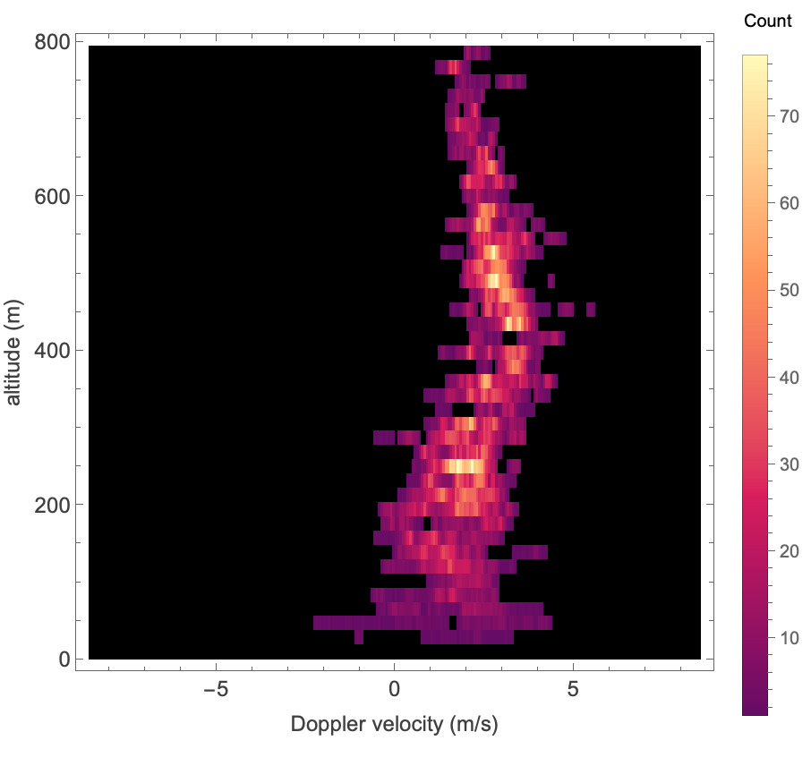 |
Marshall Bradley, "WiPPR Images of Convective Boundary Layer Turbulence" from the Wolfram Data Repository (2026)