Wolfram Data Repository
Immediate Computable Access to Curated Contributed Data
UN-adjusted gridded world population density for the years 2000, 2005, 2010, and 2015
Originator: Socioeconomic Data and Applications Center (sedac)
This dataset contains estimates of population density for the years 2000, 2005, 2010, and 2015, based on counts consistent with national censuses and population registers with respect to relative spatial distribution, but adjusted to match United Nations country totals.
Each dataset is an image, where a pixel represents a square in a lat-lon grid. The value of a pixel represents the average population density, in square kilometers, over its square. Eight different levels of granularity are provided for each year, with pixel dimensions 338×136, 675×272, 1350×544, 2700×1088, 5400×2175, 10800×4350, 21600×8700, and 43200×17400.
A particular image can be referenced by its year and zoom level (1 being the smallest and 8 being the largest). For example the image from 2005 at zoom level 4 is referenced by "Year2005Zoom4". Zoom levels 7 and 8 are broken up into 4 and 16 tiles of dimension 10800×4350, respectively. The 9th tile at zoom level 8 for the year 2010 is referenced by "Year2010Zoom8Tile9".
The longitude covered by each zoom level is -180 Degrees to 180 Degrees, and the latitude covered is -60 Degrees to 85 Degrees. Missing data is represented with -1, which is mostly over bodies of water and uninhabited areas of land.
The element "RangeData" provides the center coordinates of the leftmost, rightmost, top, and bottom squares, along with the granularity of the zoom level. The smallest zoom level has squares with side lengths 1.066 Degrees and the largest zoom level has lengths 0.00833 Degrees, which near the equator corresponds to roughly 1 square kilometer.
Retrieve the default content:
| In[1]:= |
| Out[1]= | 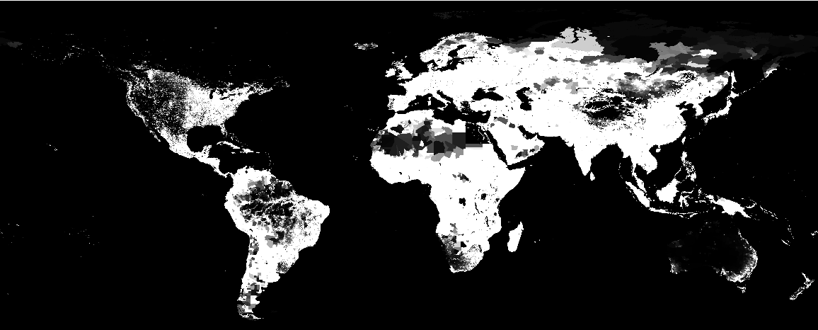 |
The data is provided as an Image:
| In[2]:= |
| Out[3]= |
Highlight areas with data white and areas missing data black:
| In[4]:= |
| Out[5]= | 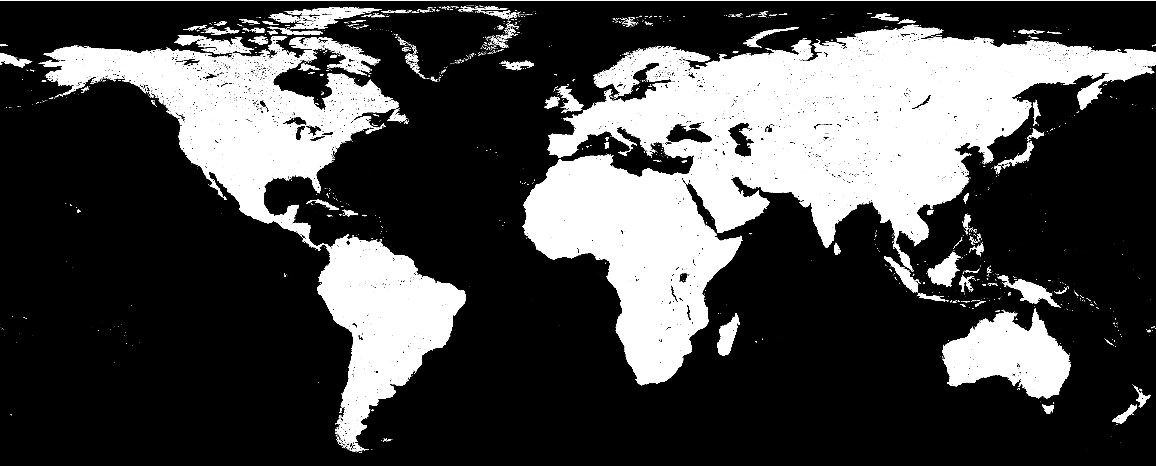 |
Create a binned heat map of world population density:
| In[6]:= | ![binf = Piecewise[{{-1, # < 0}, {0, # < 1}, {1, # < 5}, {2, # < 25}, {3, # < 250}, {4, # < 1000}}, 5] &;
data = ImageData[ResourceData["Gridded World Population Density"]];
ArrayPlot[Map[binf, data, {2}], ColorFunction -> "Rainbow", ColorRules -> {-1 -> LightGray}]](https://www.wolframcloud.com/obj/resourcesystem/images/c90/c908679c-279b-4226-822c-9040c5c8960d/303feb1e233b4212.png) |
| Out[7]= | 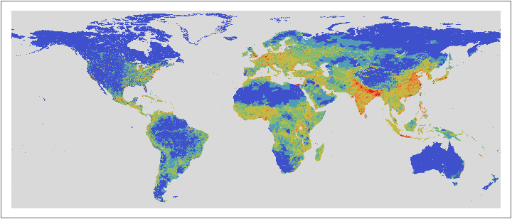 |
See the range and resolution of each tile. Here are the first six zoom levels:
| In[8]:= |
| Out[9]= | 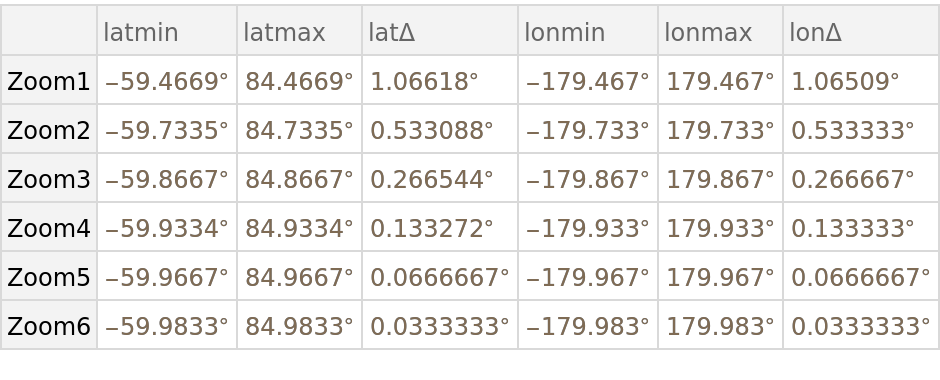 |
Wolfram Research, "Gridded World Population Density" from the Wolfram Data Repository (2018)
http://creativecommons.org/licenses/by/4.0