Examples
Basic Examples (3)
Retrieve the model:
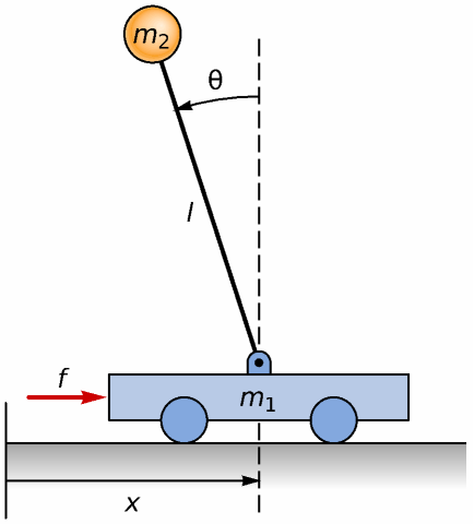
The icon:
The annotation:
Scope & Additional Elements (4)
Available content elements:
The available model types:
The operating point:
The parameters:
Visualizations (2)
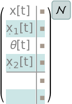
The numerical model of the system:
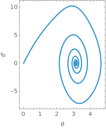
A parametric plot of the pendulum's angular position and velocity:
Analysis (3)
The numerical model:
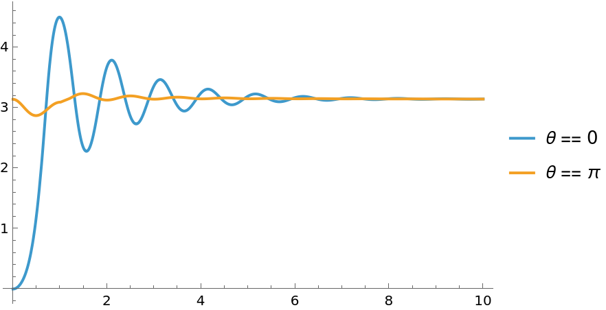
Responses starting from the upright and downright positions:
Both responses settle in the stable downward position:
Bibliographic Citation
Suba Thomas,
"Inverted Pendulum Model"
from the Wolfram Data Repository
(2025)
Data Resource History
Publisher Information


![nssm = ResourceData[\!\(\*
TagBox["\"\<Inverted Pendulum Model\>\"",
#& ,
BoxID -> "ResourceTag-Inverted Pendulum Model-Input",
AutoDelete->True]\), "NonlinearStateSpaceModel"] /. ResourceData[\!\(\*
TagBox["\"\<Inverted Pendulum Model\>\"",
#& ,
BoxID -> "ResourceTag-Inverted Pendulum Model-Input",
AutoDelete->True]\), "Parameters"]](https://www.wolframcloud.com/obj/resourcesystem/images/ce9/ce91f968-d837-4913-9060-a3f9b55a8c4e/69a063dc25cc109b.png)
![ResourceData[\!\(\*
TagBox["\"\<Inverted Pendulum Model\>\"",
#& ,
BoxID -> "ResourceTag-Inverted Pendulum Model-Input",
AutoDelete->True]\), "NonlinearStateSpaceModel"] /. ResourceData[\!\(\*
TagBox["\"\<Inverted Pendulum Model\>\"",
#& ,
BoxID -> "ResourceTag-Inverted Pendulum Model-Input",
AutoDelete->True]\), "Parameters"]](https://www.wolframcloud.com/obj/resourcesystem/images/ce9/ce91f968-d837-4913-9060-a3f9b55a8c4e/4c6bac6001d1c2f1.png)