Human Protein Atlas

Data from The Human Protein Atlas

Details

The data is based on The Human Protein Atlas version 23.0 and Ensembl version 109.

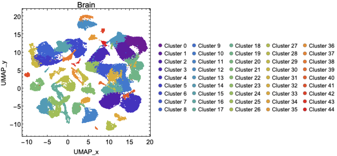
The data is covers the Tissue Atlas, Brain Atlas, Pathology Atlas, Single Cell Atlas and Subcellular Atlas.

Each dataset in the UMAP coordinates for cells is an Association of the form <|cluster id1 → {{cell id11, {UMAP_x11, UMAP_y11}}, {cell id12, {UMAP_x12, UMAP_y12}}, …, {cell id1N, {UMAP_x1N, UMAP_y1N}}}, …, cluster idM → {{cell idM1, {UMAP_xM1, UMAP_yM1}}, {cell idM2, {UMAP_xM2, UMAP_yM2}}, …, {cell idMK, {UMAP_xMK, UMAP_yMK}}}|>, where M, N, K are positive integers.

Uniform Manifold Approximation and Projection (UMAP) is a method for reducing the dimensionality of a data set (Becht E et al. (2018))

Gene and protein expression levels for different datasets are expressed as transcripts per million ("TPM"), protein-transcripts per million ("pTPM") and normalized expression ("nTPM").

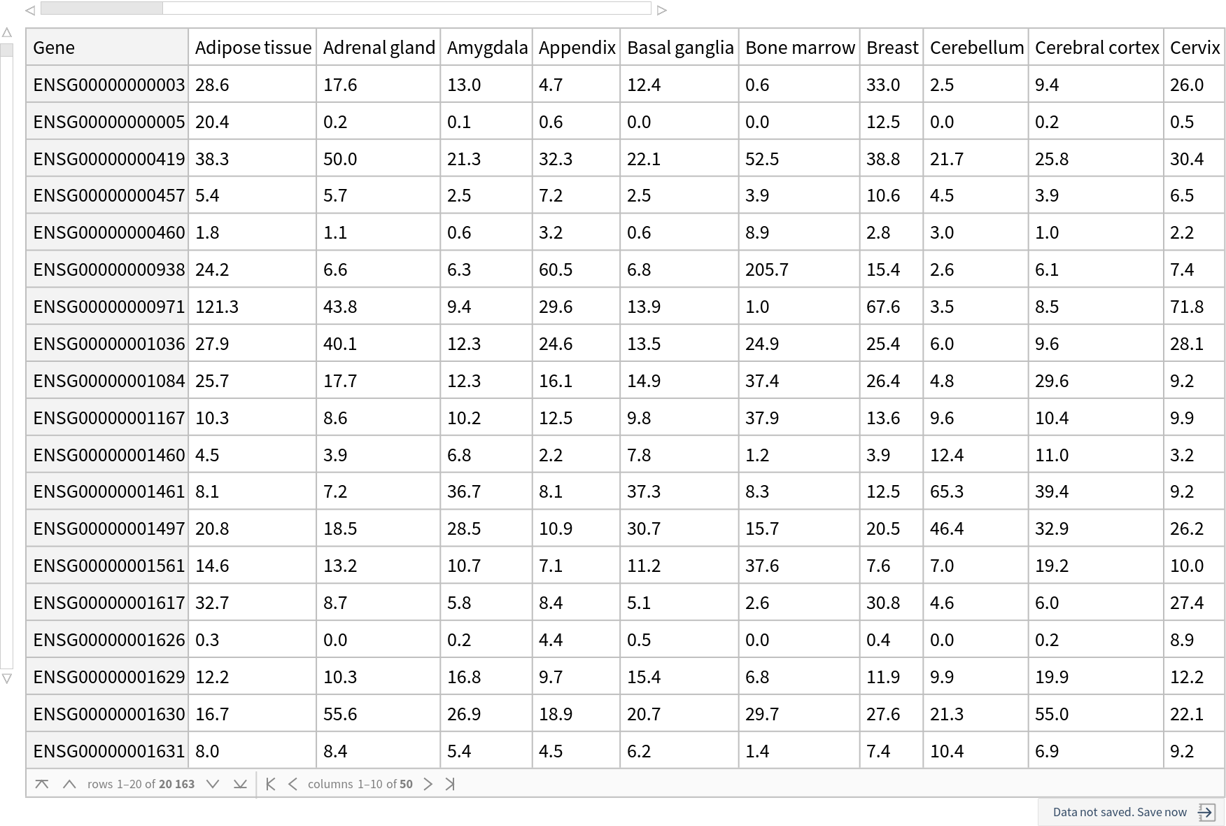
The default content is a Association containing a the expression levels (nTPM) of genes in different human tissues along with these additional data:

"TissueAtlas Gene co-expression network"

list of gene pairs with high correlation (>0.7) in expression in tissues

"TissueAtlas Gene co-expression graph"

graph of co-expressing genes in tissues

"TissueAtlas Gene co-expression network Graph measures"

graph measures for the "TissueAtlas Gene co-expression network"

"TissueAtlas maximum expression location"

maximum expression location of genes

"BrainAtlas gene expression (TPM)"

expression levels (TPM) of genes in human brain

"BrainAtlas gene expression (pTPM)"

expression levels (pTPM) of genes in human brain

"BrainAtlas gene expression (nTPM)"

expression levels (nTPM) of genes in human brain

"BrainAtlas Gene co-expression network"

list of gene pairs with high correlation (>0.7) in expression in human brain

"BrainAtlas Gene co-expression graph"

graph of co-expressing genes in human brain

"BrainAtlas Gene co-expression network Graph measures"

graph measures for the "BrainAtlas Gene co-expression network"

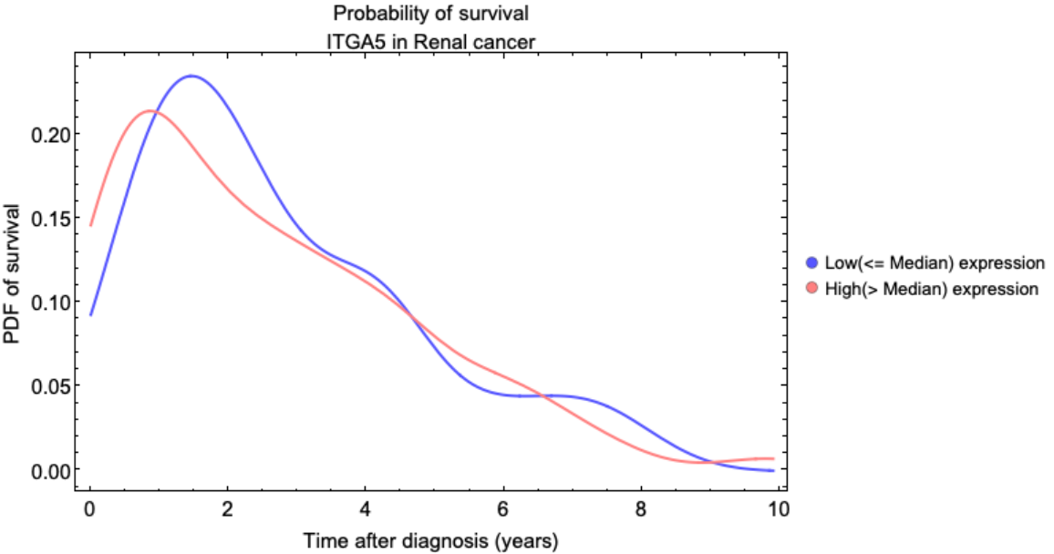
"PathologyAtlas"

data about roles of genes in different cancers

"PathologyAtlas mRNA expression (FPKM) "<>cancer

gene expression (FPKM) values for different genes in different cancer types

"PathologyAtlas Samples"

sample details for gene expression data in different cancers

"SingleCellAtlas expression (nTPM)"

expression levels (nTPM) of genes in different cell types

"SingleCellAtlas cell clusters"

description of cell clusters

"SingleCellAtlas expression in cell clusters(nTPM)"

expression levels (nTPM) of genes in different cell types and clusters

"SingleCellAtlas Gene co-expression network"

list of gene pairs with high correlation (>0.7) in expression in single cell types

"SingleCellAtlas Gene co-expression graph"

graph of co-expressing genes in different human single cell types

"SingleCellAtlas Gene co-expression network Graph measures"

graph measures for the "SingleCellAtlas Gene co-expression network"

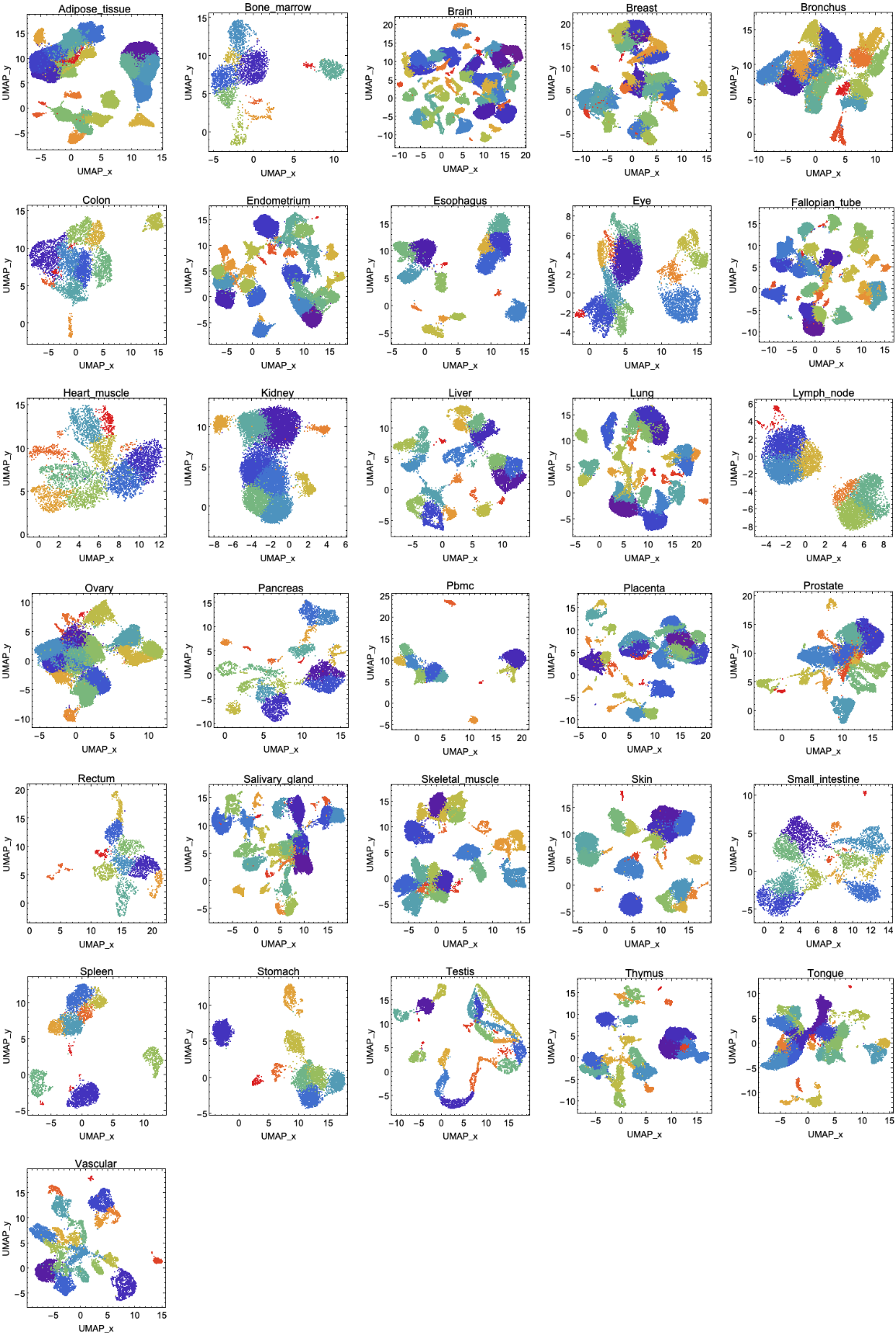
"SingleCellAtlas UMAP coordinates in tissue "<>tissue

UMAP coordinates for cells in clusters for different tissues

"SubCellularAtlas"

expression of genes in different subcellular regions

"Ensembl ID gene name association"

Association of Emsembl IDs of genes and common gene names

"Ensembl ID gene description UniProtID association"

Association of Emsembl IDs of genes to gene description and UniProtID

"Organ tissue association"

Association of organs and tissues belonging to an organ

"PathologyAtlas mRNA expression (FPKM) "<>cancer has the gene expression (FPKM) values for different genes in different cancer types for different samples in The Cancer Genome Atlas.

cancer has the following values: "BRCA","BLCA","CESC","COAD","READ","GBM","HNSC","KIRC","KIRP","KICH","LIHC","LUAD","LUSC","OV","PAAD","PRAD","SKCM","STAD","TGCT","THCA","UCEC". These are abbreviations for different cancer types

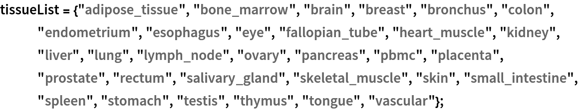
tissue for UMAP coordinates can be adipose_tissue, bone_marrow, brain, breast, bronchus, colon, endometrium, esophagus, eye, fallopian_tube, heart_muscle, kidney, liver, lung, lymph_node, ovary, pancreas, pbmc, placenta, prostate, rectum, salivary_gland, skeletal_muscle, skin, small_intestine, spleen, stomach, testis, thymus, tongue and vascular.

(20163 elements)

Examples

Basic Examples (2)

Gene expression (nTPM) in different human tissues:

In[1]:=

$Dataset@ResourceData[\!$\* TagBox["\"\<Human Protein Atlas\>\"", #& , BoxID -> "ResourceTag-Human Protein Atlas-Input", AutoDelete->True]$]$

Out[1]=

Expression of 50 strongest expressing genes in human tissues (Red color indicates data not available):

In[2]:=

$RNAExpressionData = ResourceData[\!$\* TagBox["\"\<Human Protein Atlas\>\"", #& , BoxID -> "ResourceTag-Human Protein Atlas-Input", AutoDelete->True]$]; tissues = RNAExpressionData[[1]]; ensemblIDGeneAssoc = ResourceData[\!$\* TagBox["\"\<Human Protein Atlas\>\"", #& , BoxID -> "ResourceTag-Human Protein Atlas-Input", AutoDelete->True]$, "Ensembl ID gene name association"]; ensemblIDs = Keys@RNAExpressionData[[2 ;; -1]]; genes = ensemblIDGeneAssoc /@ ensemblIDs; v = Values@RNAExpressionData; totExp = Table[Total@v[[i]] /. 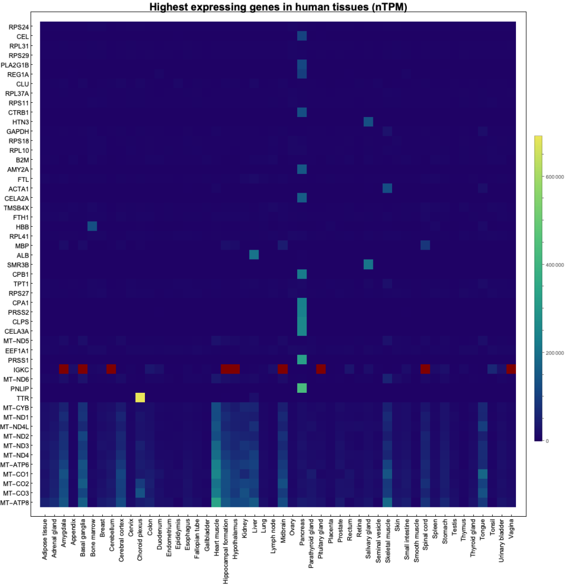{"NA" -> 0}, {i, 2, Length@genes + 1}]; sv = Sort[totExp]; numGenes = 50; pos = Flatten@ Map[Position[totExp, #] &, sv[[Length@genes - numGenes ;; Length@genes]]]; highestExpressionGenes = ensemblIDs[[pos]]; highestExpressionGeneNames = Map[ensemblIDGeneAssoc, highestExpressionGenes]; ftx = MapThread[{#1, #2} &, {Range@Length@highestExpressionGeneNames, highestExpressionGeneNames}]; fty = MapThread[{#1, Rotate[Capitalize@#2, Pi/2]} &, {Range@ Length@tissues, tissues}]; array = v[[pos + 1]]; mA = {Min@array /. "NA" -> 0, Max@array /. "NA" -> 0}; ArrayPlot[array, ColorFunction -> "BlueGreenYellow", FrameTicks -> {ftx, fty}, ImageSize -> 1000, Frame -> True, FrameStyle -> Directive[Black, 12], PlotLegends -> BarLegend[{"BlueGreenYellow", mA}], PlotLabel -> Style["Highest expressing genes in human tissues (nTPM)", Black, Bold, 20]]$

Out[18]=

Visualizations (3)

Subgraph containing 30 randomly chosen genes from the tissue co-expression network with VertexSize scaled by VertexDegree in the graph:

In[19]:=

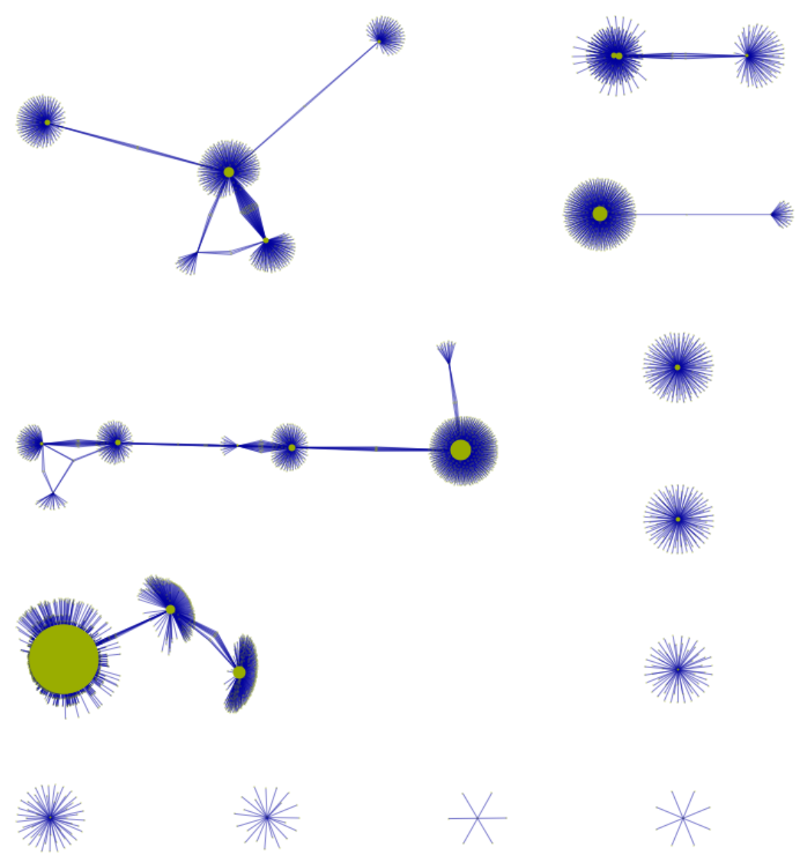
$RNACoExpressionNetwork = ResourceData[\!$\* TagBox["\"\<Human Protein Atlas\>\"", #& , BoxID -> "ResourceTag-Human Protein Atlas-Input", AutoDelete->True]$, "TissueAtlas Gene co-expression graph"]; getSubGraph[graph_Graph, vertexList_] := Graph@Sort@ DeleteDuplicates@ Flatten[IncidenceList[graph, #] & /@ vertexList]; ResourceFunction[ ResourceObject[<|"Name" -> "VertexSizeScaledGraph", "ShortName" -> "VertexSizeScaledGraph", "UUID" -> "82dfde6e-106f-4322-a329-1216e9f28362", "ResourceType" -> "Function", "Version" -> "1.1.0", "Description" -> "Visualize a graph with scaled vertex size based on custom graph related measures", "RepositoryLocation" -> URL[ "https://www.wolframcloud.com/obj/resourcesystem/api/1.0"], "SymbolName" -> "FunctionRepository`$4d8c3d76bc4e42be9489e98149696195`VertexSizeScaledGraph", "FunctionLocation" -> CloudObject[ "https://www.wolframcloud.com/obj/b0eb1e52-6cf3-4b6a-8efb-7950a9c63da5"]|>, ResourceSystemBase -> Automatic]][ getSubGraph[RNACoExpressionNetwork, Echo@RandomChoice[VertexList@RNACoExpressionNetwork, 30]], VertexStyle -> RGBColor[0.6, 0.68, 0], EdgeStyle -> RGBColor[0, 0, 0.61], "MaxVertexSize" -> 200, VertexLabels -> Placed["Name", Tooltip]]$

Out[2]=

Expression patterns of randomly chosen pair of connected genes in the "TissueAtlas Gene co-expression network":

In[20]:=

$RNAExpressionData = ResourceData[\!$\* TagBox["\"\<Human Protein Atlas\>\"", #& , BoxID -> "ResourceTag-Human Protein Atlas-Input", AutoDelete->True]$]; RNACoExpressionNetwork = ResourceData[\!$\* TagBox["\"\<Human Protein Atlas\>\"", #& , BoxID -> "ResourceTag-Human Protein Atlas-Input", AutoDelete->True]$, "TissueAtlas Gene co-expression network"]; ensemblIDGeneAssoc = ResourceData[\!$\* TagBox["\"\<Human Protein Atlas\>\"", #& , BoxID -> "ResourceTag-Human Protein Atlas-Input", AutoDelete->True]$, "Ensembl ID gene name association"]; ensemblIDs = Keys@RNAExpressionData[[2 ;; -1]]; genes = ensemblIDGeneAssoc /@ ensemblIDs; 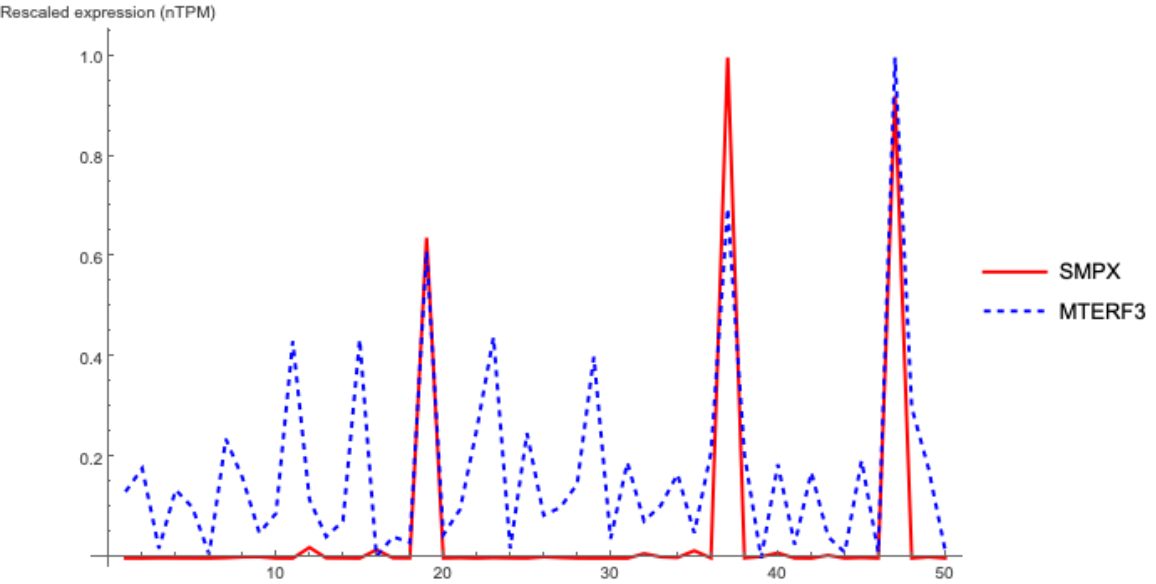genePairs = VertexList[Graph@RandomChoice@EdgeList@RNACoExpressionNetwork]; array = (Rescale@RNAExpressionData[#] &) /@ ensemblIDs[[Flatten[Position[genes, #] & /@ genePairs]]]; ListLinePlot[array, PlotLegends -> {genePairs[[1]], genePairs[[2]]}, AxesLabel -> {None, "Rescaled expression (nTPM)" }, PlotRange -> All, PlotStyle -> {Red, Directive[Blue, Dashed]}, ImageSize -> Large]$

Out[27]=

Correlation between expression levels:

In[28]:=

Out[28]=

Expression levels for a ITGA5, one of the most frequently occurring genes in unfavorable cancer prognosis, in different cancers:

Code

In[29]:=

$plotCancerShortNames = {{"GBM"}, {"THCA"}, {"LUAD", "LUSC"}, {"COAD", "READ"}, {"HNSC"}, {"STAD"}, {"LIHC"}, {"PAAD"}, {"KIRC", "KIRP", "KICH"}, {"BLCA"}, {"PRAD"}, {"TGCT"}, {"BRCA"}, {"CESC"}, {"UCEC"}, {"OV"}, {"SKCM"}}; plotCancerLongNames = {"Glioma", "Thyroid cancer", "Lung cancer", "Colorectal cancer", "Head and neck cancer", "Stomach cancer", "Liver cancer", "Pancreatic cancer", "Renal cancer", "Urothelial cancer", "Prostate cancer", "Testis cancer", "Breast cancer", "Cervical cancer", "Endometrial cancer", "Ovarian cancer", "Melanoma"}; plotCancerColors = { RGBColor[1., 0.800000094944996, 0.3019609068561773, 1.], RGBColor[ 0.454901902606013, 0.37647054361669646`, 0.5568627171197533, 1.], RGBColor[ 0.35816992186625884`, 0.48104578647795015`, 0.35294121107541104`, 1.], RGBColor[ 9.589812169208401*^-7, 0.4705881904500226, 0.7176470465066893, 1.], RGBColor[ 9.589812169208401*^-7, 0.4705881904500226, 0.7176470465066893, 1.], RGBColor[ 9.589812169208401*^-7, 0.4705881904500226, 0.7176470465066893, 1.], RGBColor[ 0.7960782989163758, 0.7686276968328074, 0.8745099497269464, 1.], RGBColor[ 0.5372548827993883, 0.7215686797169252, 0.5294118166131165, 1.], RGBColor[1., 0.509803856871976, 0.3725490654639468, 1.], RGBColor[1., 0.509803856871976, 0.3725490654639468, 1.], RGBColor[ 0.5137255717824479, 0.8196078836750866, 0.941176564576014, 1.], RGBColor[ 0.5137255717824479, 0.8196078836750866, 0.941176564576014, 1.], RGBColor[ 0.9832875177291199, 0.7011909727286483, 0.8148310349772592, 1.], RGBColor[ 0.9832875177291199, 0.7011909727286483, 0.8148310349772592, 1.], RGBColor[ 0.9832875177291199, 0.7011909727286483, 0.8148310349772592, 1.], RGBColor[ 0.9832875177291199, 0.7011909727286483, 0.8148310349772592, 1.], RGBColor[ 0.9946701221664577, 0.575625452943115, 0.3876721337241307, 1.]}; cancers = {"BRCA", "BLCA", "CESC", "COAD", "READ", "GBM", "HNSC", "KIRC", "KIRP", "KICH", "LIHC", "LUAD", "LUSC", "OV", "PAAD", "PRAD", "SKCM", "STAD", "TGCT", "THCA", "UCEC"}; pathologyData = ResourceData[\!$\* TagBox["\"\<Human Protein Atlas\>\"", #& , BoxID -> "ResourceTag-Human Protein Atlas-Input", AutoDelete->True]$, "PathologyAtlas mRNA expression (FPKM) " <> #] & /@ cancers; dataFull = AssociationThread[cancers, pathologyData];$

In[30]:=

$plotCancerColorsAssoc = AssociationThread[plotCancerLongNames, plotCancerColors]; plotCancerTickLabelsAssoc = AssociationThread[plotCancerLongNames, plotCancerShortNames]; ensGeneAssoc = ResourceData[\!$\* TagBox["\"\<Human Protein Atlas\>\"", #& , BoxID -> "ResourceTag-Human Protein Atlas-Input", AutoDelete->True]$, "Ensembl ID gene name association"]; geneEnsAssoc = AssociationThread[Values@ensGeneAssoc, Keys@ensGeneAssoc]; ticks = MapThread[{#1, Rotate[#2, -5*Pi/3]} &, {Range@ Length@plotCancerLongNames, plotCancerLongNames}]; 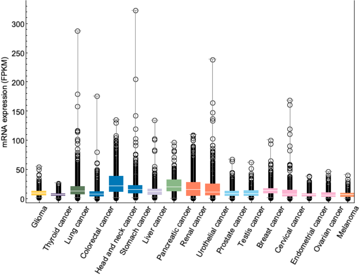cancerGeneExpressionPlot[gene_] := Module[{ensembl, data, plottingData, xVal, yVals, plotData}, ensembl = geneEnsAssoc@gene; data = (#@ensembl) & /@ dataFull; plottingData = Table[xVal = Position[plotCancerLongNames, cancerNameToPlot][[1, 1]]; yVals = Flatten[data[#] & /@ plotCancerTickLabelsAssoc[cancerNameToPlot]]; plotData = {xVal, #} & /@ yVals; {plotData, yVals}, {cancerNameToPlot, plotCancerLongNames}]; Show[ListPlot[plottingData[[All, 1]], PlotStyle -> Black, PlotMarkers -> "\!$\* GraphicsBox[CircleBox[{0, 0}], ImageSize->{11., Automatic}]$", FrameTicks -> {{Automatic, None}, {ticks, None}}, PlotRange -> Full, ImageSize -> 700, Frame -> True, FrameLabel -> {None, "mRNA expression (FPKM)"}, FrameStyle -> Directive[Black, 15]], BoxWhiskerChart[plottingData[[All, 2]], ChartStyle -> plotCancerColors]]] 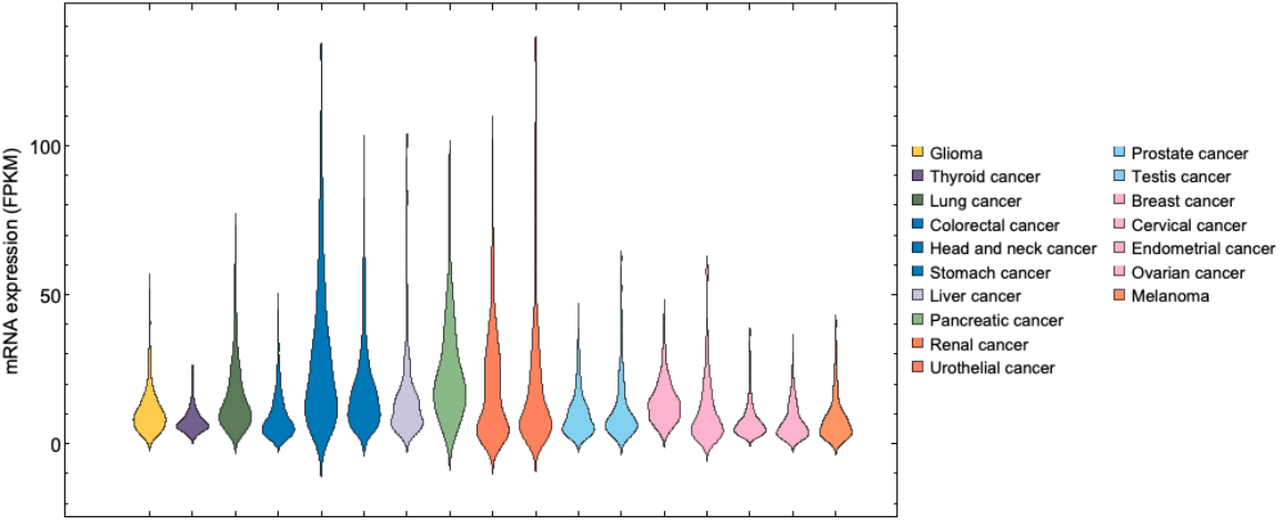cancerGeneExpressionDistributionChart[gene_] := Module[{ensembl, data, plottingData}, ensembl = geneEnsAssoc@gene; data = (#@ensembl) & /@ dataFull; plottingData = Table[xVal = Position[plotCancerLongNames, cancerNameToPlot][[1, 1]]; Flatten[ data[#] & /@ plotCancerTickLabelsAssoc[cancerNameToPlot]], {cancerNameToPlot, plotCancerLongNames}]; DistributionChart[plottingData, ChartStyle -> plotCancerColors, ChartLegends -> plotCancerLongNames, PlotRange -> Automatic, ImageSize -> 700, FrameLabel -> {None, "mRNA expression (FPKM)"}, FrameStyle -> Directive[Black, 15]]]$

Plots

In[31]:=

Out[31]=

In[32]:=

Out[32]=

Survival probability for ITGA5 in Renal cancer:

Code

In[33]:=

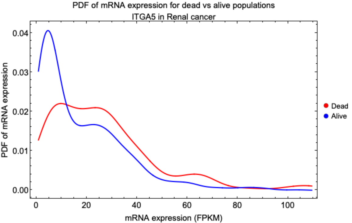
(* Evaluate this cell to get the example input *) CloudGet["https://www.wolframcloud.com/obj/9a3d4ec7-24c2-4d03-90d7-6ac26111a2da"]

Plots

In[34]:=

Out[34]=

In[35]:=

Out[35]=

In[36]:=

Out[36]=

Cell cluster plot for different tissues:

In[37]:=

$CellClusterPlot[organ_] := Module[{assoc, clusters, L, color, clusterList}, assoc = ResourceData[\!$\* TagBox["\"\<Human Protein Atlas\>\"", #& , BoxID -> "ResourceTag-Human Protein Atlas-Input", AutoDelete->True]$, "SingleCellAtlas UMAP coordinates in tissue " <> organ]; clusters = Keys@assoc; clusterList = StringJoin["Cluster ", ToString@#] & /@ clusters; L = Length@clusters; color = ColorData["Rainbow"][#] & /@ (Range[L]/L); Legended[ ListPlot[Table[Style[assoc[[i, All, -1]], color[[i]]], {i, L}], Axes -> False, FrameLabel -> {"UMAP_x", "UMAP_y"}, FrameStyle -> Directive[Black, Thickness[0.0025], 15], AspectRatio -> 1, PlotLabel -> Style[Capitalize@organ, Black, 18], Frame -> True, PlotStyle -> PointSize[Small]], SwatchLegend[color, clusterList, LegendMarkers -> "Bubble"]]]$

In[38]:=

Out[38]=

Cluster plot for all tissues:

In[39]:=

$CellClusterPlotBasic[organ_] := Module[{assoc, clusters, L, color, clusterList}, assoc = ResourceData[\!$\* TagBox["\"\<Human Protein Atlas\>\"", #& , BoxID -> "ResourceTag-Human Protein Atlas-Input", AutoDelete->True]$, "SingleCellAtlas UMAP coordinates in tissue " <> organ]; clusters = Keys@assoc; clusterList = StringJoin["Cluster ", ToString@#] & /@ clusters; L = Length@clusters; color = ColorData["Rainbow"][#] & /@ (Range[L]/L); ListPlot[Table[Style[assoc[[i, All, -1]], color[[i]]], {i, L}], Axes -> False, FrameLabel -> {"UMAP_x", "UMAP_y"}, FrameStyle -> Directive[Black, Thickness[0.0025], 15], AspectRatio -> 1, PlotLabel -> Style[Capitalize@organ, Black, 18], Frame -> True, PlotStyle -> PointSize[Small]]]$

In[40]:=

$tissueList = {"adipose_tissue", "bone_marrow", "brain", "breast", "bronchus", "colon", "endometrium", "esophagus", "eye", "fallopian_tube", "heart_muscle", "kidney", "liver", "lung", "lymph_node", "ovary", "pancreas", "pbmc", "placenta", "prostate", "rectum", "salivary_gland", "skeletal_muscle", "skin", "small_intestine", "spleen", "stomach", "testis", "thymus", "tongue", "vascular"};$

In[41]:=

In[42]:=

Out[42]=

Analysis (2)

Power law dependence of VertexDegree in the human gene co-expression networks showing its scale-free nature:

Tissue Atlas

In[43]:=

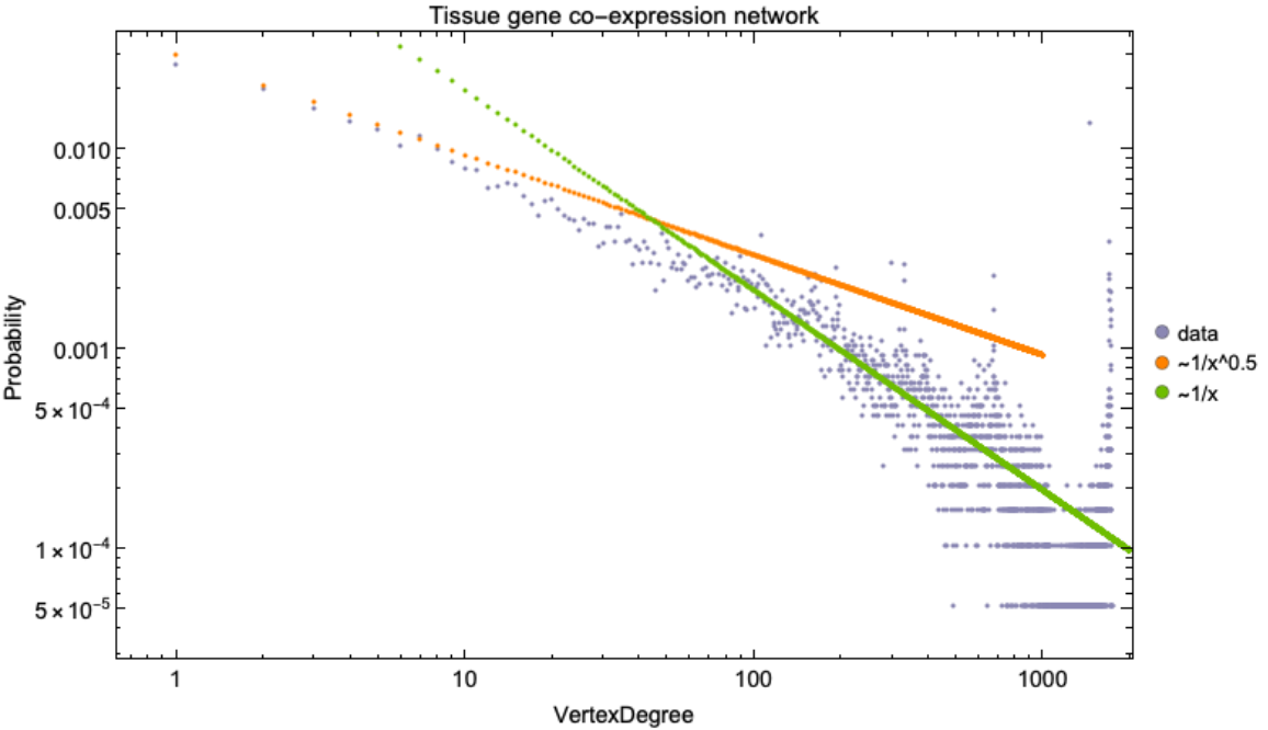
$RNACoExpressionNetwork = ResourceData[\!$\* TagBox["\"\<Human Protein Atlas\>\"", #& , BoxID -> "ResourceTag-Human Protein Atlas-Input", AutoDelete->True]$, "TissueAtlas Gene co-expression graph"]; power = 1/2; power2 = 1; Legended[Show[ListLogLogPlot[ResourceFunction[ ResourceObject[<|"Name" -> "VertexDegreeRelativeFrequencies", "ShortName" -> "VertexDegreeRelativeFrequencies", "UUID" -> "a76d6242-2a31-4326-bb6a-df4e446f50a6", "ResourceType" -> "Function", "Version" -> "1.0.0", "Description" -> "Relative frequencies of VertexDegree in a Graph", "RepositoryLocation" -> URL[ "https://www.wolframcloud.com/obj/resourcesystem/api/1.0"], "SymbolName" -> "FunctionRepository`$8f984335e1b840a0b3c49438547b6dc4`VertexDegreeRelativeFrequencies", "FunctionLocation" -> CloudObject[ "https://www.wolframcloud.com/obj/beb446d6-a18b-4eae-b8fa-c7d76afd70c6"]|>, ResourceSystemBase -> Automatic]][ RNACoExpressionNetwork], ImageSize -> 700, PlotStyle -> RGBColor[0.54, 0.53, 0.7000000000000001], Frame -> True, FrameStyle -> Directive[Black, 14], PlotLabel -> Style["Tissue gene co-expression network", Black, 15], FrameLabel -> {{"Probability", None}, {"VertexDegree", Automatic}}], ListLogLogPlot[(0.03/#^power) & /@ (Range@1000), PlotStyle -> RGBColor[1, 0.51, 0]], ListLogLogPlot[(0.2/#^power2) & /@ (Range@2000), PlotStyle -> RGBColor[0.43, 0.74, 0]]], SwatchLegend[{RGBColor[0.54, 0.53, 0.7000000000000001], RGBColor[ 1, 0.51, 0], RGBColor[0.43, 0.74, 0]}, {"data", "~1/x^0.5", "~1/x"}, LegendMarkers -> "Bubble"]]$

Out[40]=

Brain Atlas

In[44]:=

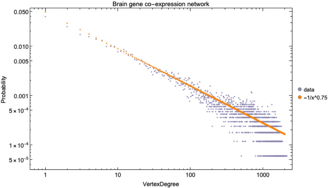
$brainGeneCoExpressionNetwork = ResourceData[\!$\* TagBox["\"\<Human Protein Atlas\>\"", #& , BoxID -> "ResourceTag-Human Protein Atlas-Input", AutoDelete->True]$, "BrainAtlas Gene co-expression graph"]; \[Alpha] = 3/4; Legended[Show[ListLogLogPlot[ResourceFunction[ ResourceObject[<|"Name" -> "VertexDegreeRelativeFrequencies", "ShortName" -> "VertexDegreeRelativeFrequencies", "UUID" -> "a76d6242-2a31-4326-bb6a-df4e446f50a6", "ResourceType" -> "Function", "Version" -> "1.0.0", "Description" -> "Relative frequencies of VertexDegree in a Graph", "RepositoryLocation" -> URL[ "https://www.wolframcloud.com/obj/resourcesystem/api/1.0"], "SymbolName" -> "FunctionRepository`$8f984335e1b840a0b3c49438547b6dc4`VertexDegreeRelativeFrequencies", "FunctionLocation" -> CloudObject[ "https://www.wolframcloud.com/obj/beb446d6-a18b-4eae-b8fa-c7d76afd70c6"]|>, ResourceSystemBase -> Automatic]][ brainGeneCoExpressionNetwork], ImageSize -> 700, PlotStyle -> RGBColor[0.54, 0.53, 0.7000000000000001], Frame -> True, FrameStyle -> Directive[Black, 14], FrameLabel -> {{"Probability", None}, {"VertexDegree", Automatic}}, PlotLabel -> Style["Brain gene co-expression network", Black, 15]], ListLogLogPlot[(0.05/#^\[Alpha]) & /@ (Range@2000), PlotStyle -> RGBColor[1, 0.51, 0]]], SwatchLegend[{RGBColor[0.54, 0.53, 0.7000000000000001], RGBColor[ 1, 0.51, 0]}, {"data", "~1/x^0.75"}, LegendMarkers -> "Bubble"]]$

Out[45]=

Single cell atlas

In[46]:=

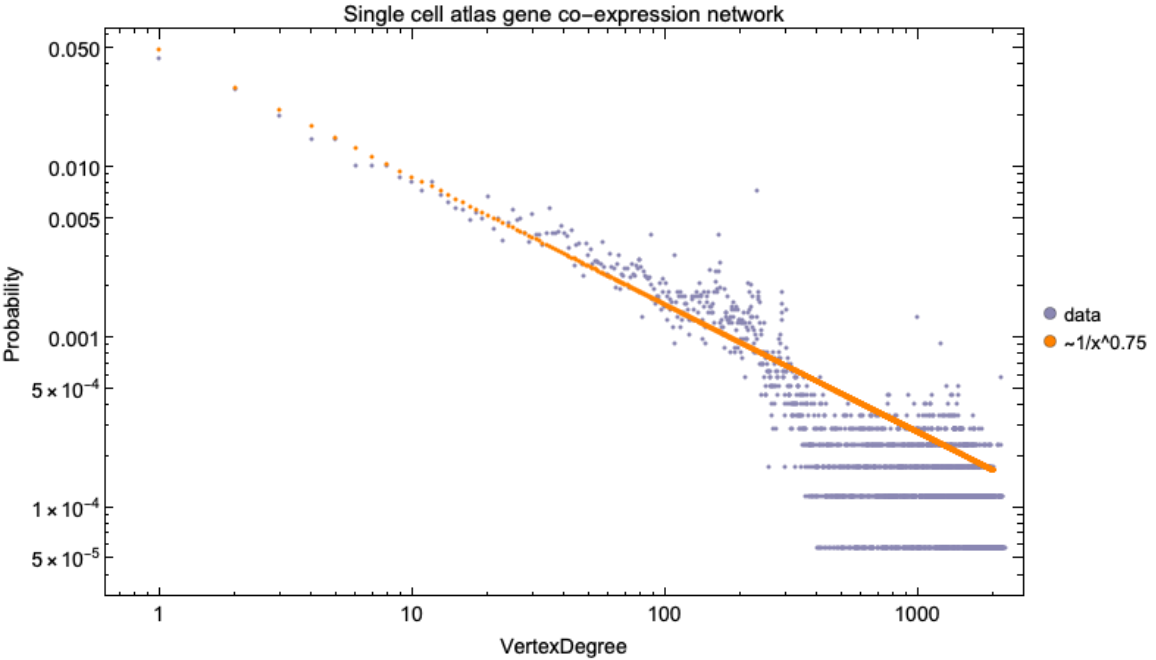
$scGeneCoExpressionNetwork = ResourceData[\!$\* TagBox["\"\<Human Protein Atlas\>\"", #& , BoxID -> "ResourceTag-Human Protein Atlas-Input", AutoDelete->True]$, "SingleCellAtlas Gene co-expression graph"]; \[Alpha] = 3/4; Legended[Show[ListLogLogPlot[ResourceFunction[ ResourceObject[<|"Name" -> "VertexDegreeRelativeFrequencies", "ShortName" -> "VertexDegreeRelativeFrequencies", "UUID" -> "a76d6242-2a31-4326-bb6a-df4e446f50a6", "ResourceType" -> "Function", "Version" -> "1.0.0", "Description" -> "Relative frequencies of VertexDegree in a Graph", "RepositoryLocation" -> URL[ "https://www.wolframcloud.com/obj/resourcesystem/api/1.0"], "SymbolName" -> "FunctionRepository`$8f984335e1b840a0b3c49438547b6dc4`VertexDegreeRelativeFrequencies", "FunctionLocation" -> CloudObject[ "https://www.wolframcloud.com/obj/beb446d6-a18b-4eae-b8fa-c7d76afd70c6"]|>, ResourceSystemBase -> Automatic]][ scGeneCoExpressionNetwork], ImageSize -> 700, PlotStyle -> RGBColor[0.54, 0.53, 0.7000000000000001], Frame -> True, FrameStyle -> Directive[Black, 14], FrameLabel -> {{"Probability", None}, {"VertexDegree", Automatic}}, PlotLabel -> Style["Single cell atlas gene co-expression network", Black, 15]], ListLogLogPlot[(0.05/#^\[Alpha]) & /@ (Range@2000), PlotStyle -> RGBColor[1, 0.51, 0]]], SwatchLegend[{RGBColor[0.54, 0.53, 0.7000000000000001], RGBColor[ 1, 0.51, 0]}, {"data", "~1/x^0.75"}, LegendMarkers -> "Bubble"]]$

Out[47]=

Visualize the values of VertexDegree and BetweennessCentrality for common genes in the three networks:

In[48]:=

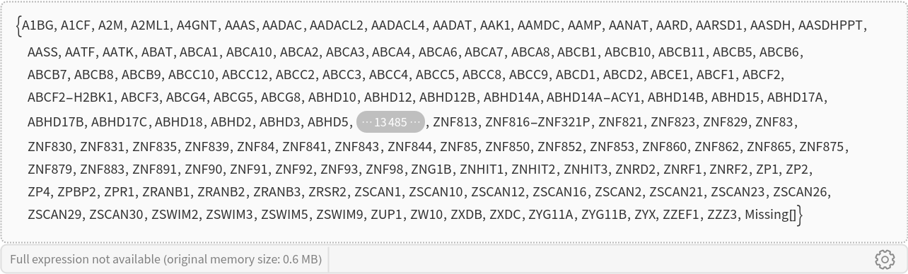
$commonGenes = Intersection[VertexList@ResourceData[\!$\* TagBox["\"\<Human Protein Atlas\>\"", #& , BoxID -> "ResourceTag-Human Protein Atlas-Input", AutoDelete->True]$, "TissueAtlas Gene co-expression graph"], VertexList@ResourceData[\!$\* TagBox["\"\<Human Protein Atlas\>\"", #& , BoxID -> "ResourceTag-Human Protein Atlas-Input", AutoDelete->True]$, "BrainAtlas Gene co-expression graph"], VertexList@ResourceData[\!$\* TagBox["\"\<Human Protein Atlas\>\"", #& , BoxID -> "ResourceTag-Human Protein Atlas-Input", AutoDelete->True]$, "SingleCellAtlas Gene co-expression graph"]]$

Out[48]=

In[49]:=

$tissueData = ResourceData[\!$\* TagBox["\"\<Human Protein Atlas\>\"", #& , BoxID -> "ResourceTag-Human Protein Atlas-Input", AutoDelete->True]$, "TissueAtlas Gene co-expression network Graph measures"]; brainData = ResourceData[\!$\* TagBox["\"\<Human Protein Atlas\>\"", #& , BoxID -> "ResourceTag-Human Protein Atlas-Input", AutoDelete->True]$, "BrainAtlas Gene co-expression network Graph measures"]; scData = ResourceData[\!$\* TagBox["\"\<Human Protein Atlas\>\"", #& , BoxID -> "ResourceTag-Human Protein Atlas-Input", AutoDelete->True]$, "SingleCellAtlas Gene co-expression network Graph measures"]; maxV = Max@ MapThread[#1* #2* #3 &, {Map[tissueData[#, "VertexDegree"] &, commonGenes], Map[brainData[#, "VertexDegree"] &, commonGenes], Map[scData[#, "VertexDegree"] &, commonGenes]}]; plotVDData = MapThread[ Tooltip[Style[{#1, #2, #3}, ColorData["Rainbow"][Log[#1* #2* #3]/Log@maxV]], #4] &, {Map[ tissueData[#, "VertexDegree"] &, commonGenes], Map[brainData[#, "VertexDegree"] &, commonGenes], Map[scData[#, "VertexDegree"] &, commonGenes], commonGenes}];$

In[50]:=

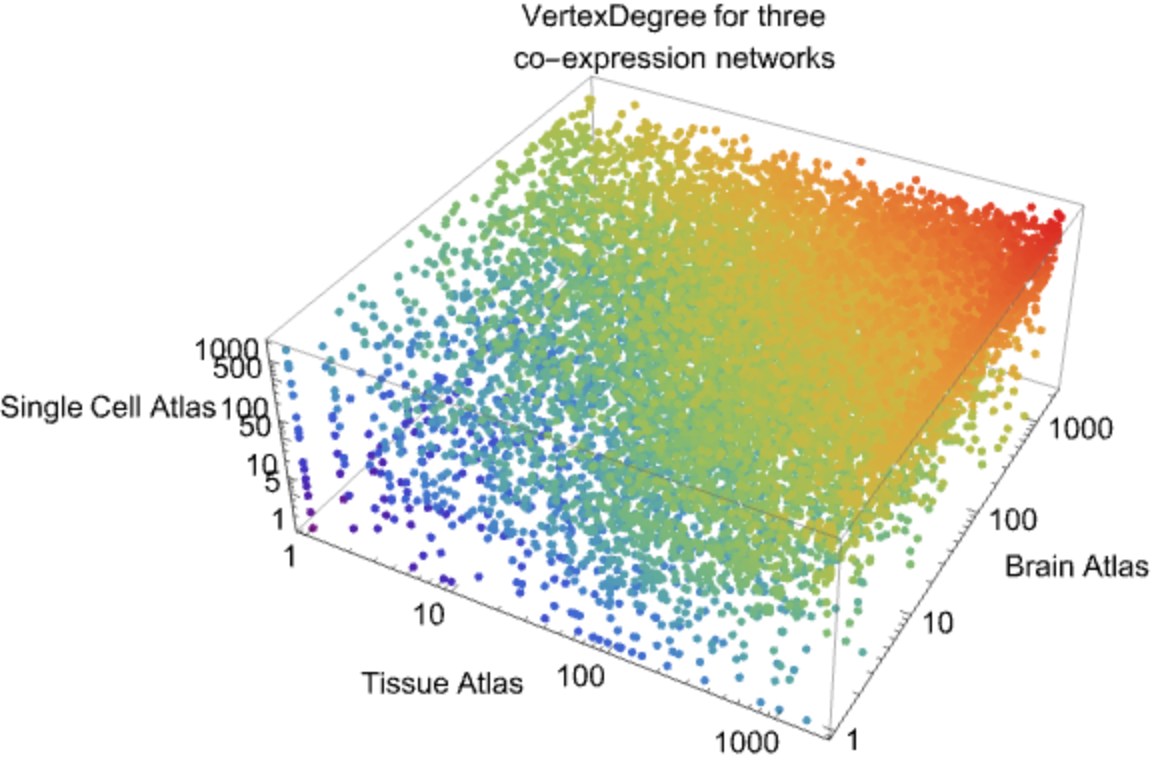
$ListPointPlot3D[plotVDData, ScalingFunctions -> {"Log", "Log", "Log"}, PlotStyle -> PointSize[Medium], AxesStyle -> Directive[Black, 15], AxesLabel -> {"Tissue Atlas", "Brain Atlas", "Single Cell Atlas"}, ImageSize -> Large, PlotLabel -> Style["VertexDegree for three\nco-expression networks", Black, 15]]$

Out[50]=

In[51]:=

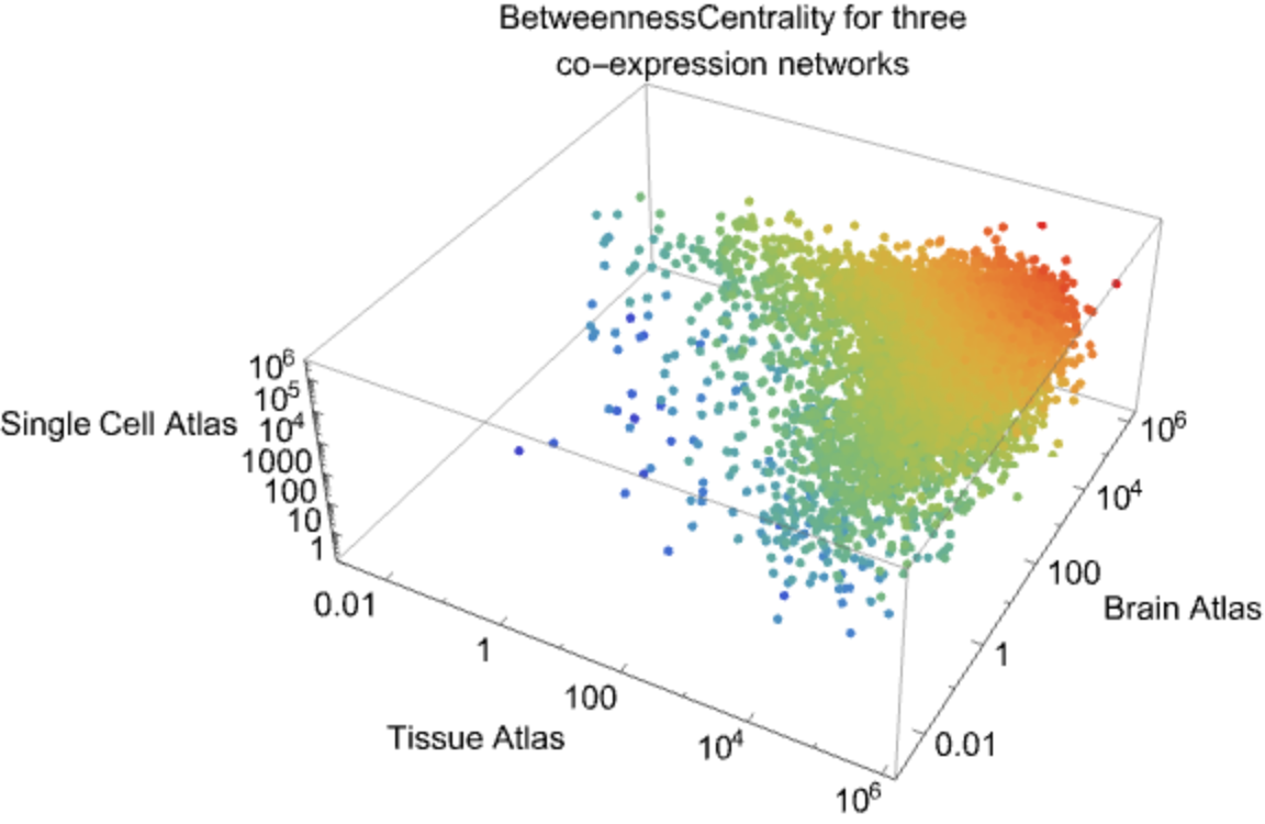
$maxV = Max@ MapThread[#1* #2* #3 &, {Map[ tissueData[#, "BetweennessCentrality"] &, commonGenes], Map[brainData[#, "BetweennessCentrality"] &, commonGenes], Map[scData[#, "BetweennessCentrality"] &, commonGenes]}]; plotBCData = MapThread[ Tooltip[Style[{#1, #2, #3}, ColorData["Rainbow"][ Log[If[#1* #2* #3 == 0, 0.000001, #1* #2* #3]]/ Log@maxV]], #4] &, {Map[ tissueData[#, "BetweennessCentrality"] &, commonGenes], Map[brainData[#, "BetweennessCentrality"] &, commonGenes], Map[scData[#, "BetweennessCentrality"] &, commonGenes], commonGenes}]; ListPointPlot3D[plotBCData, ScalingFunctions -> {"Log", "Log", "Log"}, PlotStyle -> PointSize[Medium], AxesStyle -> Directive[Black, 15], AxesLabel -> {"Tissue Atlas", "Brain Atlas", "Single Cell Atlas"}, ImageSize -> Large, PlotLabel -> Style["BetweennessCentrality for three\nco-expression networks", Black, 15]]$

Out[33]=

External Links

Bibliographic Citation

WolframChemistry, "Human Protein Atlas" from the Wolfram Data Repository (2025)

Data Resource History

Date Created: 12 November 2024

Source Metadata

Citation:
- Uhlén M et al., Tissue-based map of the human proteome. Science (2015) PubMed: 25613900 DOI: 10.1126/science.1260419
- Thul PJ et al., A subcellular map of the human proteome. Science. (2017) PubMed: 28495876 DOI: 10.1126/science.aal3321
- Sjöstedt E et al., An atlas of the protein-coding genes in the human, pig, and mouse brain. Science. (2020) PubMed: 32139519 DOI: 10.1126/science.aay5947
- Karlsson M et al., A single-cell type transcriptomics map of human tissues. Sci Adv. (2021) PubMed: 34321199 DOI: 10.1126/sciadv.abh2169
- Uhlen M et al., A pathology atlas of the human cancer transcriptome. Science. (2017) PubMed: 28818916 DOI: 10.1126/science.aan2507
- Uhlen M et al., A genome-wide transcriptomic analysis of protein-coding genes in human blood cells. Science. (2019) PubMed: 31857451 DOI: 10.1126/science.aax9198
- Sjöstedt E et al., An atlas of the protein-coding genes in the human, pig, and mouse brain. Science. (2020) PubMed: 32139519 DOI: 10.1126/science.aay5947
- Uhlén M et al., The human secretome. Sci Signal. (2019) PubMed: 31772123 DOI: 10.1126/scisignal.aaz0274
- Becht, Etienne, et al. "Dimensionality reduction for visualizing single-cell data using UMAP." Nature biotechnology 37.1 (2019): 38-44.

Data Downloads

Publisher Information

Prepared for the Wolfram Data Repository By: Soutick Saha
Publisher of Record: WolframChemistry