Wolfram Data Repository
Immediate Computable Access to Curated Contributed Data
Standard illuminants, colorimetric observer curves, and daylight components for working with visible light spectra and illumination, from Publication CIE 15:2004
| "CIE1964" | CIE 1964 Colorimetric Observer Functions (default) |
| "CIE1931" | CIE 1931 Colorimetric Observer Functions |
| "IlluminantA" | Standard Illuminant A |
| "IlluminantD65" | Standard Illuminant D65 |
| "DaylightS0S1S2" | D Series Spectral Power Distributions |
(81 elements)
Retrieve the default data, the CIE Color Matching Functions ![]() :
:
| In[1]:= | ![CIE1964 = ResourceData[\!\(\*
TagBox["\"\<Selected CIE Colorimetric Tables\>\"",
#& ,
BoxID -> "ResourceTag-Selected CIE Colorimetric Tables-Input",
AutoDelete->True]\)];
ListPlot[{CIE1964[[All, {1, 2}]], CIE1964[[All, {1, 3}]], CIE1964[[All, {1, 4}]]}, PlotLabel -> "CIE 1964 Color Matching Functions", AxesLabel -> {"\[Lambda] (nm)", ""}, PlotLegends -> Placed[{"\!\(\*OverscriptBox[\(x\), \(_\)]\)(\[Lambda])", "\!\(\*OverscriptBox[\(y\), \(_\)]\)(\[Lambda])", "\!\(\*OverscriptBox[\(z\), \(_\)]\)(\[Lambda])"}, {{0.85, 0.98}, {1, 1}}
]]](https://www.wolframcloud.com/obj/resourcesystem/images/de0/de0f6807-c051-4d6f-b0e1-562e1b62d3fa/14532136c1ef11be.png) |
| Out[2]= | 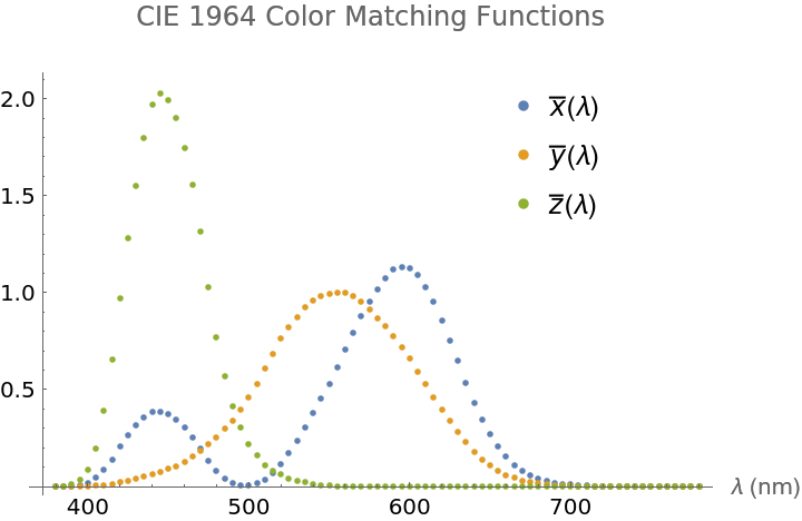 |
The standard illuminants are spectra for studying lighting. Illuminant A represents indoor, incandescent lighting, with the power spectrum of a black body at 2856° Kelvin. Illuminant D65 represents daylight at 6504° Kelvin. The relative spectral power distributions, S0, S1, and S2 of the Illuminant D series can be used to compose alternate illuminant variations.
| In[3]:= | ![CIE1931 = ResourceData[\!\(\*
TagBox["\"\<Selected CIE Colorimetric Tables\>\"",
#& ,
BoxID -> "ResourceTag-Selected CIE Colorimetric Tables-Input",
AutoDelete->True]\), "CIE1931"];
SIA = ResourceData[\!\(\*
TagBox["\"\<Selected CIE Colorimetric Tables\>\"",
#& ,
BoxID -> "ResourceTag-Selected CIE Colorimetric Tables-Input",
AutoDelete->True]\), "IlluminantA"];
SID65 = ResourceData[\!\(\*
TagBox["\"\<Selected CIE Colorimetric Tables\>\"",
#& ,
BoxID -> "ResourceTag-Selected CIE Colorimetric Tables-Input",
AutoDelete->True]\), "IlluminantD65"];
S0S1S2 = ResourceData[\!\(\*
TagBox["\"\<Selected CIE Colorimetric Tables\>\"",
#& ,
BoxID -> "ResourceTag-Selected CIE Colorimetric Tables-Input",
AutoDelete->True]\), "DaylightS0S1S2"];](https://www.wolframcloud.com/obj/resourcesystem/images/de0/de0f6807-c051-4d6f-b0e1-562e1b62d3fa/75e38d6875a73f23.png) |
| In[4]:= | ![ListPlot[{CIE1931[[All, {1, 2}]], CIE1931[[All, {1, 3}]], CIE1931[[All, {1, 4}]]}, PlotLabel -> "CIE 1931 Color Matching Functions", AxesLabel -> {"\[Lambda] (nm)", ""}, PlotLegends -> Placed[{"\!\(\*OverscriptBox[\(x\), \(_\)]\)(\[Lambda])", "\!\(\*OverscriptBox[\(y\), \(_\)]\)(\[Lambda])", "\!\(\*OverscriptBox[\(z\), \(_\)]\)(\[Lambda])"}, {{0.85, 0.98}, {1, 1}}
]]](https://www.wolframcloud.com/obj/resourcesystem/images/de0/de0f6807-c051-4d6f-b0e1-562e1b62d3fa/071ed949819f3b32.png) |
| Out[4]= | 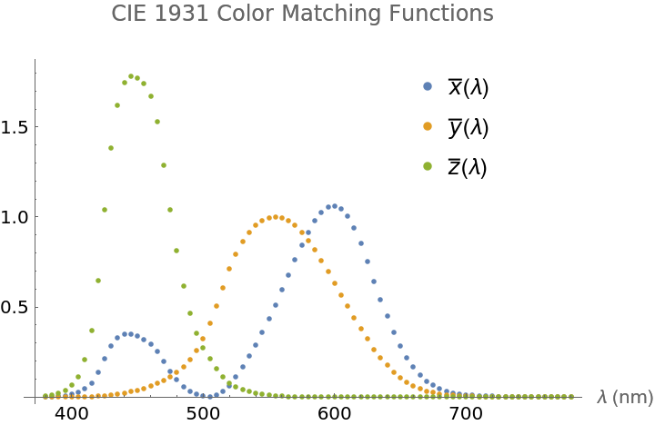 |
| In[5]:= | ![ListPlot[{S0S1S2[[All, {1, 2}]], S0S1S2[[All, {1, 3}]], S0S1S2[[All, {1, 4}]]}, PlotLabel -> "Spectral Power Distributions:\nD Series Illuminant", AxesLabel -> {"\[Lambda] (nm)", ""}, PlotLegends -> Placed[{"S0(\[Lambda])", "S1(\[Lambda])", "S2(\[Lambda])"}, {{0.925, 0.99}, {1, 1}}
]]](https://www.wolframcloud.com/obj/resourcesystem/images/de0/de0f6807-c051-4d6f-b0e1-562e1b62d3fa/6718218c57b610e1.png) |
| Out[5]= | 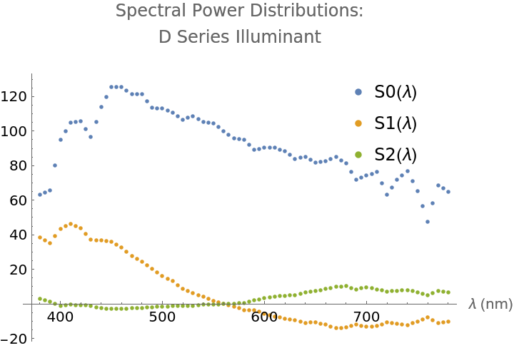 |
| In[6]:= | ![ListPlot[{SID65, SIA}, PlotLabel -> "CIE Standard Illuminants", AxesLabel -> {"\[Lambda] (nm)", ""}, PlotLegends -> Placed[{"Illuminant D65", "Illuminant A"}, {{0.425, 0.99}, {1, 1}}
]]](https://www.wolframcloud.com/obj/resourcesystem/images/de0/de0f6807-c051-4d6f-b0e1-562e1b62d3fa/4ea34088964680a4.png) |
| Out[6]= | 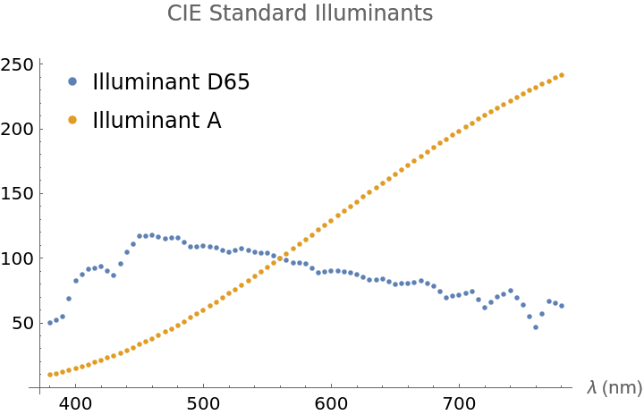 |
Converting a visible spectrum to a color is a matter of integrating the spectrum with each of the three CIE observer functions to get the CIE XYZ coordinates. Mathematica can interpret these with XYZColor[]. It is important to normalize the integrals by the integrals of the observer functions. The resulting XYZ values will represent an irradiance that is probably very bright and would just look white, so we want to normalize the color itself by dividing by Y. As expected, the daylight is cool and the incandescent 'warm'.
| In[7]:= | ![stdD65 = Interpolation[SID65];
stdA = Interpolation[SIA];
CIEX = Interpolation[CIE1964[[All, 1 ;; 2]]];
CIEY = Interpolation[CIE1964[[All, {1, 3}]]];
CIEZ = Interpolation[CIE1964[[All, {1, 4}]]];
Plot[{stdD65[w]/120, stdA[w]/120, CIEX[w], CIEY[w], CIEZ[w]}, {w, 380,
780}, PlotTheme -> "Minimal", PlotLabel -> "Integrate Standard Illuminants to XYZ Color", PlotStyle -> {{Thickness[0.015], LightBlue}, {Thickness[0.015], LightOrange}, Red, Green, Blue}, ImageSize -> Large,
PlotLegends -> Placed[{"Illuminant D65", "Illuminant A", "CIE 1964 \!\(\*OverscriptBox[\(x\), \(_\)]\)(\[Lambda])", "\!\(\*OverscriptBox[\(y\), \(_\)]\)(\[Lambda])", "\!\(\*OverscriptBox[\(z\), \(_\)]\)(\[Lambda])"}, {0.48, 0.75}],
Epilog -> First[Plot[-0.05, {w, 380, 780}, ColorFunction -> (ColorData["VisibleSpectrum", "ColorFunction"][#] &), ColorFunctionScaling -> False, Filling -> Axis, FillingStyle -> Automatic ]]]](https://www.wolframcloud.com/obj/resourcesystem/images/de0/de0f6807-c051-4d6f-b0e1-562e1b62d3fa/2fb0e6e8a24f279d.png) |
| Out[12]= | 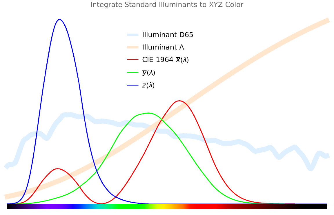 |
| In[13]:= | ![NormCIE = NIntegrate[{ CIEX[w], CIEY[w], CIEZ[w]}, {w, 380, 780}];
XYZ = NIntegrate[{ stdD65[w]*CIEX[w], stdD65[w]*CIEY[w], stdD65[w]*CIEZ[w]}, {w, 380, 780}]/NormCIE;
ColorSID65 = XYZColor[XYZ/XYZ[[2]]];
XYZ = NIntegrate[{ stdA[w]*CIEX[w], stdA[w]*CIEY[w], stdA[w]*CIEZ[w]}, {w, 380, 780}]/NormCIE;
ColorSIA = XYZColor[XYZ/XYZ[[2]]];
Graphics[{ColorSID65, Rectangle[{-1.5, -1.5}, {1.5, 1.5}], ColorSIA, Disk[]}]](https://www.wolframcloud.com/obj/resourcesystem/images/de0/de0f6807-c051-4d6f-b0e1-562e1b62d3fa/7f65280cfce8e7b2.png) |
| Out[14]= | 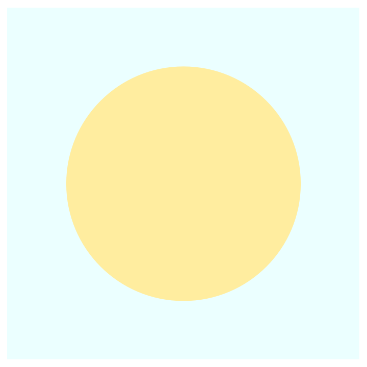 |
Arnito Lappe, "Selected CIE Colorimetric Tables" from the Wolfram Data Repository (2021)